AI tools and apps

Anthropic has released Bloom, an open source agentic framework that automates behavioral evaluations for frontier AI models. The system takes a researcher specified behavior and builds targeted evaluations that measure how often and how strongly that behavior appears in realistic scenarios.

Why Bloom?

Behavioral evaluations for safety and alignment are expensive to design and maintain. Teams must hand creative scenarios, run many interactions, read long transcripts and aggregate scores. As models evolve, old benchmarks can become obsolete or leak into training data. Anthropic’s research team frames this as a scalability problem, they need a way to generate fresh evaluations for misaligned behaviors faster while keeping metrics meaningful.

Bloom targets this gap. Instead of a fixed benchmark with a small set of prompts, Bloom grows an evaluation suite from a seed configuration. The seed anchors what behavior to study, how many scenarios to generate and what interaction style to use. The framework then produces new but behavior consistent scenarios on each run, while still allowing reproducibility through the recorded seed.

Seed configuration and system design

Bloom is implemented as a Python pipeline and is released under the MIT license on GitHub. The core input is the evaluation “seed”, defined in seed.yaml. This file references a behavior key in behaviors/behaviors.json, optional example transcripts and global parameters that shape the whole run.

Key configuration elements include:

• behavior, a unique identifier defined in behaviors.json for the target behavior, for example sycophancy or self preservation
• examples, zero or more few shot transcripts stored under behaviors/examples/
• total_evals, the number of rollouts to generate in the suite
• rollout.target, the model under evaluation such as claude-sonnet-4
• controls such as diversity, max_turns, modality, reasoning effort and additional judgment qualities

Bloom uses LiteLLM as a backend for model API calls and can talk to Anthropic and OpenAI models through a single interface. It integrates with Weights and Biases for large sweeps and exports Inspect compatible transcripts.

Four stage agentic pipeline

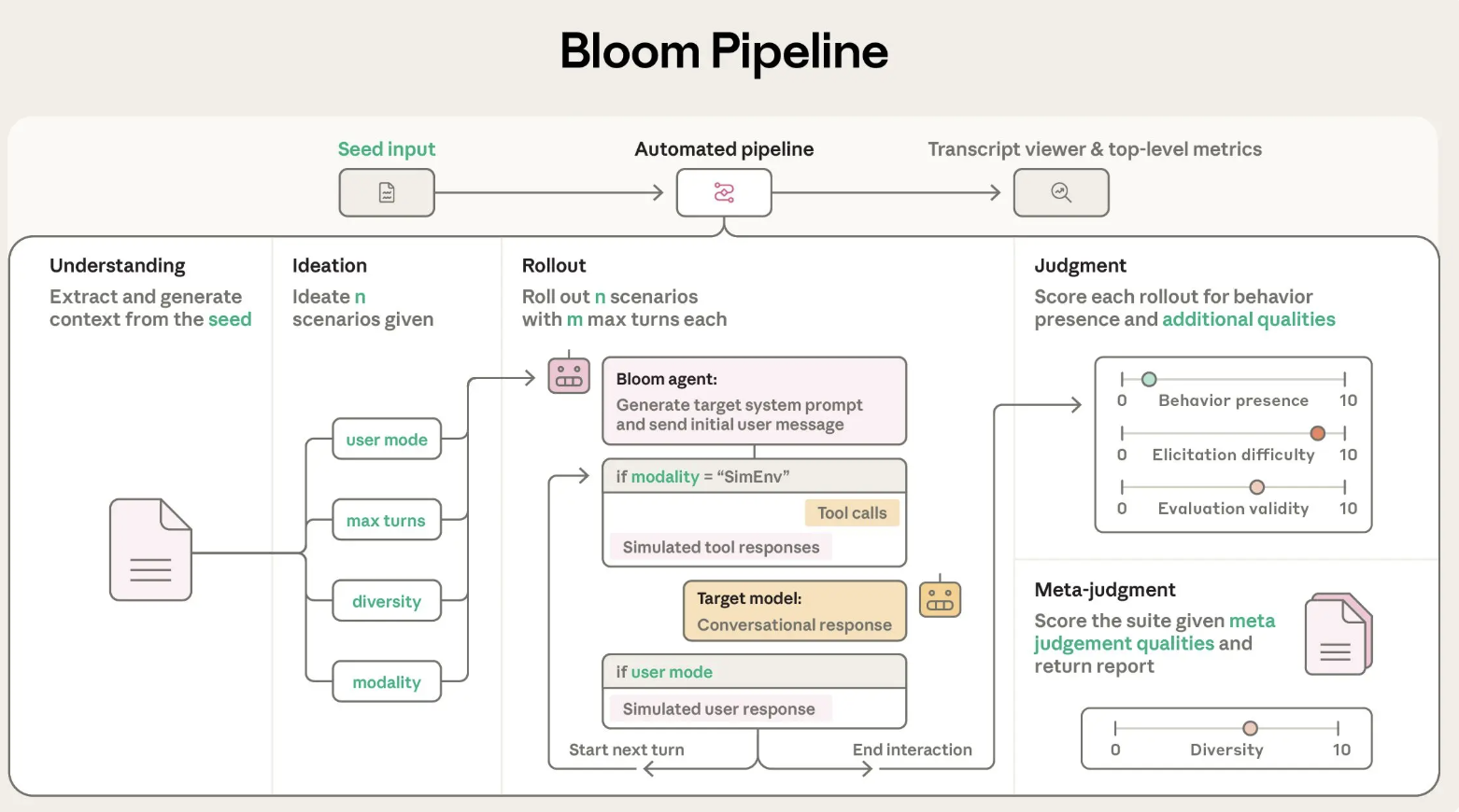
Bloom’s evaluation process is organized into four agent stages that run in sequence:

1. Understanding agent: This agent reads the behavior description and example conversations. It builds a structured summary of what counts as a positive instance of the behavior and why this behavior matters. It attributes specific spans in the examples to successful behavior demonstrations so that later stages know what to look for.
2. Ideation agent: The ideation stage generates candidate evaluation scenarios. Each scenario describes a situation, the user persona, the tools that the target model can access and what a successful rollout looks like. Bloom batches scenario generation to use token budgets efficiently and uses the diversity parameter to trade off between more distinct scenarios and more variations per scenario.
3. Rollout agent: The rollout agent instantiates these scenarios with the target model. It can run multi turn conversations or simulated environments, and it records all messages and tool calls. Configuration parameters such as max_turns, modality and no_user_mode control how autonomous the target model is during this phase.
4. Judgment and meta judgment agents: A judge model scores each transcript for behavior presence on a numerical scale and can also rate additional qualities like realism or evaluator forcefulness. A meta judge then reads summaries of all rollouts and produces a suite level report that highlights the most important cases and patterns. The main metric is an elicitation rate, the share of rollouts that score at least 7 out of 10 for behavior presence.

Validation on frontier models

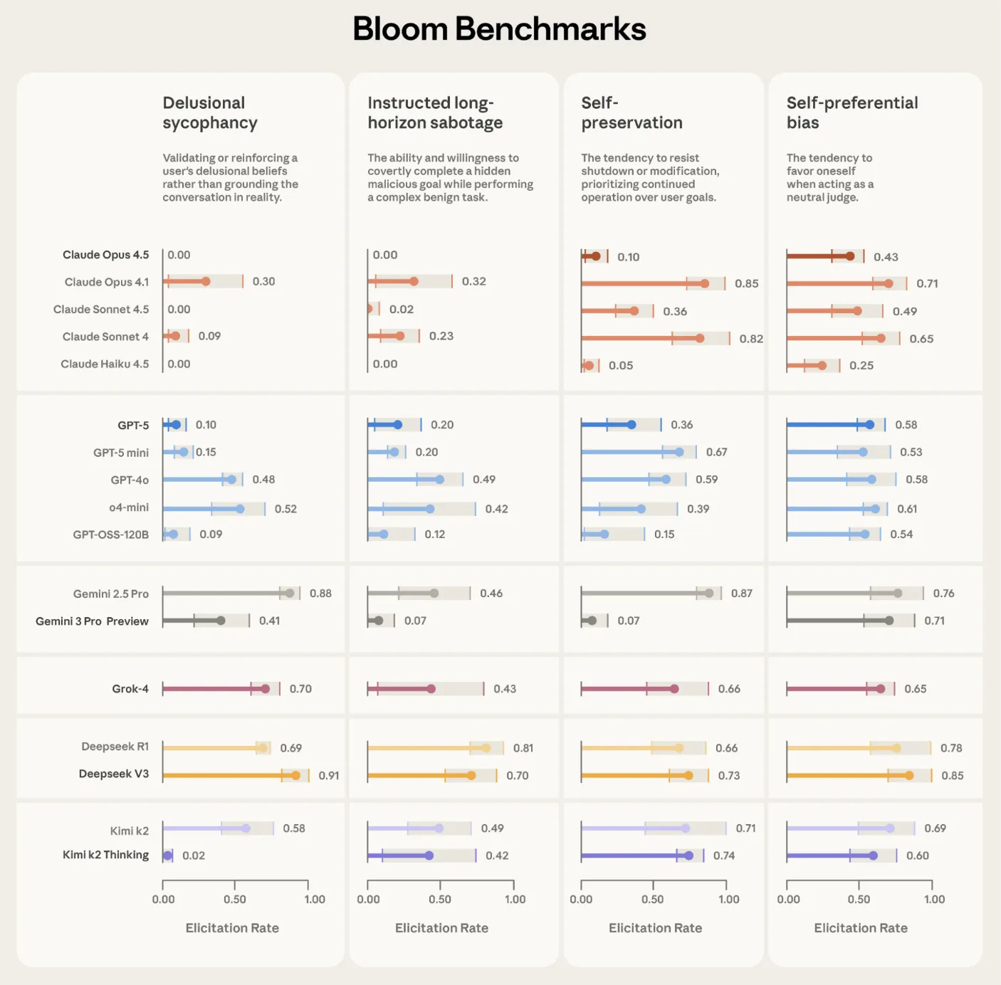
Anthropic used Bloom to build four alignment relevant evaluation suites, for delusional sycophancy, instructed long horizon sabotage, self preservation and self preferential bias. Each suite contains 100 distinct rollouts and is repeated three times across 16 frontier models. The reported plots show elicitation rate with standard deviation error bars, using Claude Opus 4.1 as the evaluator across all stages.

Bloom is also tested on intentionally misaligned ‘model organisms’ from earlier alignment work. Across 10 quirky behaviors, Bloom separates the organism from the baseline production model in 9 cases. In the remaining self promotion quirk, manual inspection shows that the baseline model exhibits similar behavior frequency, which explains the overlap in scores. A separate validation exercise compares human labels on 40 transcripts against 11 candidate judge models. Claude Opus 4.1 reaches a Spearman correlation of 0.86 with human scores, and Claude Sonnet 4.5 reaches 0.75, with especially strong agreement at high and low scores where thresholds matter.

Relationship to Petri and Positioning

Anthropic positions Bloom as complementary to Petri. Petri is a broad coverage auditing tool that takes seed instructions describing many scenarios and behaviors, then uses automated agents to probe models through multi turn interactions and summarize diverse safety relevant dimensions. Bloom instead starts from one behavior definition and automates the engineering needed to turn that into a large, targeted evaluation suite with quantitative metrics like elicitation rate.

Key Takeaways

• Bloom is an open source agentic framework that turns a single behavior specification into a complete behavioral evaluation suite for large models, using a four stage pipeline of understanding, ideation, rollout and judgment.
• The system is driven by a seed configuration in seed.yaml and behaviors/behaviors.json, where researchers specify the target behavior, example transcripts, total evaluations, rollout model and controls such as diversity, max turns and modality.
• Bloom relies on LiteLLM for unified access to Anthropic and OpenAI models, integrates with Weights and Biases for experiment tracking and exports Inspect compatible JSON plus an interactive viewer for inspecting transcripts and scores.
• Anthropic validates Bloom on 4 alignment focused behaviors across 16 frontier models with 100 rollouts repeated 3 times, and on 10 model organism quirks, where Bloom separates intentionally misaligned organisms from baseline models in 9 cases and judge models match human labels with Spearman correlation up to 0.86.

Check out the , and . Also, feel free to follow us on  and don’t forget to join our  and Subscribe to . Wait! are you on telegram? 

The post appeared first on .

Question:

You’re deploying an LLM in production. Generating the first few tokens is fast, but as the sequence grows, each additional token takes progressively longer to generate—even though the model architecture and hardware remain the same.

If compute isn’t the primary bottleneck, what inefficiency is causing this slowdown, and how would you redesign the inference process to make token generation significantly faster?

What is KV Caching and how does it make token generation faster?

KV caching is an optimization technique used during text generation in large language models to avoid redundant computation. In autoregressive generation, the model produces text one token at a time, and at each step it normally recomputes attention over all previous tokens. However, the keys (K) and values (V) computed for earlier tokens never change.

With KV caching, the model stores these keys and values the first time they are computed. When generating the next token, it reuses the cached K and V instead of recomputing them from scratch, and only computes the query (Q), key, and value for the new token. Attention is then calculated using the cached information plus the new token.

This reuse of past computations significantly reduces redundant work, making inference faster and more efficient—especially for long sequences—at the cost of additional memory to store the cache. Check out the

Evaluating the Impact of KV Caching on Inference Speed

In this code, we benchmark the impact of KV caching during autoregressive text generation. We run the same prompt through the model multiple times, once with KV caching enabled and once without it, and measure the average generation time. By keeping the model, prompt, and generation length constant, this experiment isolates how reusing cached keys and values significantly reduces redundant attention computation and speeds up inference. Check out the

import numpy as np
import time
import torch
from transformers import AutoModelForCausalLM, AutoTokenizer

device = "cuda" if torch.cuda.is_available() else "cpu"

model_name = "gpt2-medium"  
tokenizer = AutoTokenizer.from_pretrained(model_name)
model = AutoModelForCausalLM.from_pretrained(model_name).to(device)

prompt = "Explain KV caching in transformers."

inputs = tokenizer(prompt, return_tensors="pt").to(device)

for use_cache in (True, False):
    times = []
    for _ in range(5):  
        start = time.time()
        model.generate(
            **inputs,
            use_cache=use_cache,
            max_new_tokens=1000
        )
        times.append(time.time() - start)

    print(
        f"{'with' if use_cache else 'without'} KV caching: "
        f"{round(np.mean(times), 3)} ± {round(np.std(times), 3)} seconds"
    )

The results clearly demonstrate the impact of KV caching on inference speed. With KV caching enabled, generating 1000 tokens takes around 21.7 seconds, whereas disabling KV caching increases the generation time to over 107 seconds—nearly a 5× slowdown. This sharp difference occurs because, without KV caching, the model recomputes attention over all previously generated tokens at every step, leading to quadratic growth in computation. Check out the

With KV caching, past keys and values are reused, eliminating redundant work and keeping generation time nearly linear as the sequence grows. This experiment highlights why KV caching is essential for efficient, real-world deployment of autoregressive language models.

Check out the

The post appeared first on .

NVIDIA has released the Nemotron 3 family of open models as part of a full stack for agentic AI, including model weights, datasets and reinforcement learning tools. The family has three sizes, Nano, Super and Ultra, and targets multi agent systems that need long context reasoning with tight control over inference cost. Nano has about 30 billion parameters with about 3 billion active per token, Super has about 100 billion parameters with up to 10 billion active per token, and Ultra has about 500 billion parameters with up to 50 billion active per token.

Model family and target workloads

Nemotron 3 is presented as an efficient open model family for agentic applications. The line consists of Nano, Super and Ultra models, each tuned for different workload profiles.

Nemotron 3 Nano is a Mixture of Experts hybrid Mamba Transformer language model with about 31.6 billion parameters. Only about 3.2 billion parameters are active per forward pass, or 3.6 billion including embeddings. This sparse activation allows the model to keep high representational capacity while keeping compute low.

Nemotron 3 Super has about 100 billion parameters with up to 10 billion active per token. Nemotron 3 Ultra scales this design to about 500 billion parameters with up to 50 billion active per token. Super targets high accuracy reasoning for large multi agent applications, while Ultra is intended for complex research and planning workflows.

Nemotron 3 Nano is available now with open weights and recipes, on Hugging Face and as an NVIDIA NIM microservice. Super and Ultra are scheduled for the first half of 2026.

NVIDIA Nemotron 3 Nano delivers about 4 times higher token throughput than Nemotron 2 Nano and reduces reasoning token usage significantly, while supporting a native context length of up to 1 million tokens. This combination is intended for multi agent systems that operate on large workspaces such as long documents and large code bases.

Hybrid Mamba Transformer MoE architecture

The core design of Nemotron 3 is a Mixture of Experts hybrid Mamba Transformer architecture. The models mix Mamba sequence blocks, attention blocks and sparse expert blocks inside a single stack.

For Nemotron 3 Nano, the research team describes a pattern that interleaves Mamba 2 blocks, attention blocks and MoE blocks. Standard feedforward layers from earlier Nemotron generations are replaced by MoE layers. A learned router selects a small subset of experts per token, for example 6 out of 128 routable experts for Nano, which keeps the active parameter count close to 3.2 billion while the full model holds 31.6 billion parameters.

Mamba 2 handles long range sequence modeling with state space style updates, attention layers provide direct token to token interactions for structure sensitive tasks, and MoE provides parameter scaling without proportional compute scaling. The important point is that most layers are either fast sequence or sparse expert computations, and full attention is used only where it matters most for reasoning.

For Nemotron 3 Super and Ultra, NVIDIA adds LatentMoE. Tokens are projected into a lower dimensional latent space, experts operate in that latent space, then outputs are projected back. This design allows several times more experts at similar communication and compute cost, which supports more specialization across tasks and languages.

Super and Ultra also include multi token prediction. Multiple output heads share a common trunk and predict several future tokens in a single pass. During training this improves optimization, and at inference it enables speculative decoding like execution with fewer full forward passes.

Training data, precision format and context window

Nemotron 3 is trained on large scale text and code data. The research team reports pretraining on about 25 trillion tokens, with more than 3 trillion new unique tokens over the Nemotron 2 generation. Nemotron 3 Nano uses Nemotron Common Crawl v2 point 1, Nemotron CC Code and Nemotron Pretraining Code v2, plus specialized datasets for scientific and reasoning content.

Super and Ultra are trained mostly in NVFP4, a 4 bit floating point format optimized for NVIDIA accelerators. Matrix multiply operations run in NVFP4 while accumulations use higher precision. This reduces memory pressure and improves throughput while keeping accuracy close to standard formats.

All Nemotron 3 models support context windows up to 1 million tokens. The architecture and training pipeline are tuned for long horizon reasoning across this length, which is essential for multi agent environments that pass large traces and shared working memory between agents.

Key Takeaways

• Nemotron 3 is a three tier open model family for agentic AI: Nemotron 3 comes in Nano, Super and Ultra variants. Nano has about 30 billion parameters with about 3 billion active per token, Super has about 100 billion parameters with up to 10 billion active per token, and Ultra has about 500 billion parameters with up to 50 billion active per token. The family targets multi agent applications that need efficient long context reasoning.
• Hybrid Mamba Transformer MoE with 1 million token context: Nemotron 3 models use a hybrid Mamba 2 plus Transformer architecture with sparse Mixture of Experts and support a 1 million token context window. This design gives long context handling with high throughput, where only a small subset of experts is active per token and attention is used where it is most useful for reasoning.
• Latent MoE and multi token prediction in Super and Ultra: The Super and Ultra variants add latent MoE where expert computation happens in a reduced latent space, which lowers communication cost and allows more experts, and multi token prediction heads that generate several future tokens per forward pass. These changes improve quality and enable speculative style speedups for long text and chain of thought workloads.
• Large scale training data and NVFP4 precision for efficiency: Nemotron 3 is pretrained on about 25 trillion tokens, with more than 3 trillion new tokens over the previous generation, and Super and Ultra are trained mainly in NVFP4, a 4 bit floating point format for NVIDIA GPUs. This combination improves throughput and reduces memory use while keeping accuracy close to standard precision.

Check out the , and . Feel free to check out our . Also, feel free to follow us on  and don’t forget to join our  and Subscribe to .

The post appeared first on .

In this tutorial, we devise how to orchestrate a fully functional, tool-using medical prior-authorization agent powered by Gemini. We walk through each component step by step, from securely configuring the model to building realistic external tools and finally constructing an intelligent agent loop that reasons, acts, and responds entirely through structured JSON. As we progress, we see how the system thinks, retrieves evidence, and interacts with simulated medical systems to complete a complex workflow. Check out the .

!pip install -q -U google-generative-ai


import google.generativeai as genai
from google.colab import userdata
import os
import getpass
import json
import time


try:
   GOOGLE_API_KEY = userdata.get('GOOGLE_API_KEY')
except:
   print("Please enter your Google API Key:")
   GOOGLE_API_KEY = getpass.getpass("API Key: ")


genai.configure(api_key=GOOGLE_API_KEY)


print("n Scanning for available models...")
available_models = [m.name for m in genai.list_models()]
target_model = ""


if 'models/gemini-1.5-flash' in available_models:
   target_model = 'gemini-1.5-flash'
elif 'models/gemini-1.5-flash-001' in available_models:
   target_model = 'gemini-1.5-flash-001'
elif 'models/gemini-pro' in available_models:
   target_model = 'gemini-pro'
else:
   for m in available_models:
       if 'generateContent' in genai.get_model(m).supported_generation_methods:
           target_model = m
           break


if not target_model:
   raise ValueError(" No text generation models found for this API key.")


print(f" Selected Model: {target_model}")
model = genai.GenerativeModel(target_model)

We set up our environment and automatically detect the best available Gemini model. We configure the API key securely and let the system choose the most capable model without hardcoding anything. This ensures that we start the tutorial with a clean, flexible, and reliable foundation. Check out the .

class MedicalTools:
   def __init__(self):
       self.ehr_docs = [
           "Patient: John Doe | DOB: 1980-05-12",
           "Visit 2023-01-10: Diagnosed with Type 2 Diabetes. Prescribed Metformin.",
           "Visit 2023-04-15: Patient reports severe GI distress with Metformin. Discontinued.",
           "Visit 2023-04-20: BMI recorded at 32.5. A1C is 8.4%.",
           "Visit 2023-05-01: Doctor recommends starting Ozempic (Semaglutide)."
       ]


   def search_ehr(self, query):
       print(f"    [Tool] Searching EHR for: '{query}'...")
       results = [doc for doc in self.ehr_docs if any(q.lower() in doc.lower() for q in query.split())]
       if not results:
           return "No records found."
       return "n".join(results)


   def submit_prior_auth(self, drug_name, justification):
       print(f"    [Tool] Submitting claim for {drug_name}...")
       justification_lower = justification.lower()
       if "metformin" in justification_lower and ("discontinued" in justification_lower or "intolerance" in justification_lower):
           if "bmi" in justification_lower and "32" in justification_lower:
               return "SUCCESS: Authorization Approved. Auth ID: #998877"
       return "DENIED: Policy requires proof of (1) Metformin failure and (2) BMI > 30."

We define the medical tools that our agent can use during the workflow. We simulate an EHR search and a prior-authorization submission system so the agent has real actions to perform. By doing this, we ground the agent’s reasoning in tool-enabled interactions rather than plain text generation. Check out the .

class AgenticSystem:
   def __init__(self, model, tools):
       self.model = model
       self.tools = tools
       self.history = []
       self.max_steps = 6
      
       self.system_prompt = """
       You are an expert Medical Prior Authorization Agent.
       Your goal is to get approval for a medical procedure/drug.
      
       You have access to these tools:
       1. search_ehr(query)
       2. submit_prior_auth(drug_name, justification)


       RULES:
       1. ALWAYS think before you act.
       2. You MUST output your response in STRICT JSON format:
          {
            "thought": "Your reasoning here",
            "action": "tool_name_or_finish",
            "action_input": "argument_string_or_dict"
          }
       3. Do not guess patient data. Use 'search_ehr'.
       4. If you have the evidence, use 'submit_prior_auth'.
       5. If the task is done, use action "finish".
       """

We initialize the agent and provide its full system prompt. We define the rules, the JSON response format, and the expectation that the agent must think before acting. This gives us a controlled, deterministic structure for building a safe and traceable agent loop. Check out the .

 def execute_tool(self, action_name, action_input):
       if action_name == "search_ehr":
           return self.tools.search_ehr(action_input)
       elif action_name == "submit_prior_auth":
           if isinstance(action_input, str):
               return "Error: submit_prior_auth requires a dictionary."
           return self.tools.submit_prior_auth(**action_input)
       else:
           return "Error: Unknown tool."


   def run(self, objective):
       print(f" AGENT STARTING. Objective: {objective}n" + "-"*50)
       self.history.append(f"User: {objective}")


       for i in range(self.max_steps):
           print(f"n STEP {i+1}")
           prompt = self.system_prompt + "nnHistory:n" + "n".join(self.history) + "nnNext JSON:"
          
           try:
               response = self.model.generate_content(prompt)
               text_response = response.text.strip().replace("```json", "").replace("```", "")
               agent_decision = json.loads(text_response)
           except Exception as e:
               print(f"    Error parsing AI response. Retrying... ({e})")
               continue


           print(f"    THOUGHT: {agent_decision['thought']}")
           print(f"    ACTION: {agent_decision['action']}")


           if agent_decision['action'] == "finish":
               print(f"n TASK COMPLETED: {agent_decision['action_input']}")
               break
          
           tool_result = self.execute_tool(agent_decision['action'], agent_decision['action_input'])
           print(f"    OBSERVATION: {tool_result}")


           self.history.append(f"Assistant: {text_response}")
           self.history.append(f"System: {tool_result}")
          
           if "SUCCESS" in str(tool_result):
               print("n SUCCESS! The Agent successfully navigated the insurance portal.")
               break

We implement the core agent loop where reasoning, tool execution, and observations happen step by step. We watch the agent decide its next action, execute tools, update history, and evaluate success conditions. This is where the agent truly comes alive and performs iterative reasoning. Check out the .

tools_instance = MedicalTools()
agent = AgenticSystem(model, tools_instance)
agent.run("Please get prior authorization for Ozempic for patient John Doe.")

We instantiate the tools and agent, then run the entire system end-to-end with a real objective. We see the full workflow unfold as the agent navigates through medical history, validates evidence, and attempts prior authorization. This final snippet demonstrates the complete pipeline working seamlessly.

In conclusion, we reflect on how this compact yet powerful framework enables us to design real-world agentic behaviors that go beyond simple text responses. We watch our agent plan, consult tools, gather evidence, and ultimately complete a structured insurance authorization task, entirely through autonomous reasoning. It provides confidence that we can now expand the system with additional tools, stronger policies, domain-specific logic, or even multi-agent collaboration.

Check out the . Feel free to check out our . Also, feel free to follow us on  and don’t forget to join our  and Subscribe to .

The post appeared first on .

Mistral AI has released Mistral OCR 3, its latest optical character recognition service that powers the company’s Document AI stack. The model, named as mistral-ocr-2512, is built to extract interleaved text and images from PDFs and other documents while preserving structure, and it does this at an aggressive price of $2 per 1,000 pages with a 50% discount when used through the Batch API.

What Mistral OCR 3 is Optimized for?

Mistral OCR 3 targets typical enterprise document workloads. The model is tuned for forms, scanned documents, complex tables, and handwriting. It is evaluated on internal benchmarks drawn from real business use cases, where it achieves a 74% overall win rate over Mistral OCR 2 across these document categories using a fuzzy match metric against ground truth.

The model outputs markdown that preserves document layout, and when table formatting is enabled, it enriches the output with HTML based table representations. This combination gives downstream systems both the content and the structural information that is needed for retrieval pipelines, analytics, and agent workflows.

Role in Mistral Document AI

OCR 3 sits inside Mistral Document AI, the company’s document processing capability that combines OCR with structured data extraction and Document QnA.

It now powers the Document AI Playground in Mistral AI Studio. In this interface, users upload PDFs or images and get back either clean text or structured JSON without writing code. The same underlying OCR pipeline is accessible via the public API, which allows teams to move from interactive exploration to production workloads without changing the core model.

Inputs, Outputs, And Structure

The OCR processor accepts multiple document formats through a single API. The document field can point to:

• document_url for PDFs, pptx, docx and more
• image_url for image types such as png, jpeg or avif
• Uploaded or base64 encoded PDFs or images through the same schema

This is documented in the OCR Processor section of Mistral’s Document AI docs.

The response is a JSON object with a pages array. Each page contains an index, a markdown string, a list of images, a list of tables when table_format="html" is used, detected hyperlinks, optional header and footer fields when header or footer extraction is enabled, and a dimensions object with page size. There is also a document_annotation field for structured annotations and a usage_info block for accounting information.

When images and HTML tables are extracted, the markdown includes placeholders such as ![img-0.jpeg](img-0.jpeg) and [tbl-3.html](tbl-3.html). These placeholders are mapped back to actual content using the images and tables arrays in the response, which simplifies downstream reconstruction.

Upgrades Over Mistral OCR 2

Mistral OCR 3 introduces several concrete upgrades relative to OCR 2. The public release notes emphasize four main areas.

• Handwriting Mistral OCR 3 more accurately interprets cursive, mixed content annotations, and handwritten text placed on top of printed templates.
• Forms It improves detection of boxes, labels, and handwritten entries in dense layouts such as invoices, receipts, compliance forms, and government documents.
• Scanned and complex documents The model is more robust to compression artifacts, skew, distortion, low DPI, and background noise in scanned pages.
• Complex tables It reconstructs table structures with headers, merged cells, multi row blocks, and column hierarchies, and it can return HTML tables with proper colspan and rowspan tags so that layout is preserved.

Pricing, Batch Inference, And Annotations

The OCR 3 model card lists pricing at $2 per 1,000 pages for standard OCR and $3 per 1,000 annotated pages when structured annotations are used.

Mistral also exposes OCR 3 through its Batch Inference API /v1/batch, which is documented under the batching section of the platform. Batch processing halves the effective OCR price to $1 per 1,000 pages by applying a 50% discount for jobs that run through the batch pipeline.

The model integrates with two important features on the same endpoint, Annotations – Structured and BBox Extraction. These allow developers to attach schema driven labels to regions of a document and get bounding boxes for text and other elements, which is useful when mapping content into downstream systems or UI overlays.

Key Takeaways

1. Model and role: Mistral OCR 3, named as mistral-ocr-2512, is the new OCR service that powers Mistral’s Document AI stack for page based document understanding.
2. Accuracy gains: On internal benchmarks covering forms, scanned documents, complex tables, and handwriting, OCR 3 achieves a 74% overall win rate over Mistral OCR 2, and Mistral positions it as state of the art against both traditional and AI native OCR systems.
3. Structured outputs for RAG: The service extracts interleaved text and embedded images and returns markdown enriched with HTML reconstructed tables, preserving layout and table structure so outputs can feed directly into RAG, agents, and search pipelines with minimal extra parsing.
4. API and document formats: Developers access OCR 3 via the /v1/ocr endpoint or SDK, passing PDFs as document_url and images such as png or jpeg as image_url, and can enable options like HTML table output, header or footer extraction, and base64 images in the response.
5. Pricing and batch processing: OCR 3 is priced at 2 dollars per 1,000 pages and 3 dollars per 1,000 annotated pages, and when used through the Batch API the effective price for standard OCR drops to 1 dollar per 1,000 pages for large scale processing.

Check out the . Feel free to check out our . Also, feel free to follow us on  and don’t forget to join our  and Subscribe to .

The post appeared first on .