January 1, 2026
AI Labor Is Boring. AI Lust Is Big Business
After years of hype about generative AI increasing productivity and making lives easier, 2025 was the year erotic chatbots defined AI’s narrative.
 January 1, 2026
After years of hype about generative AI increasing productivity and making lives easier, 2025 was the year erotic chatbots defined AI’s narrative.
 December 31, 2025
Dating apps and AI companies have been touting bot wingmen for months. But the future might just be good old-fashioned meet-cutes.
 December 31, 2025
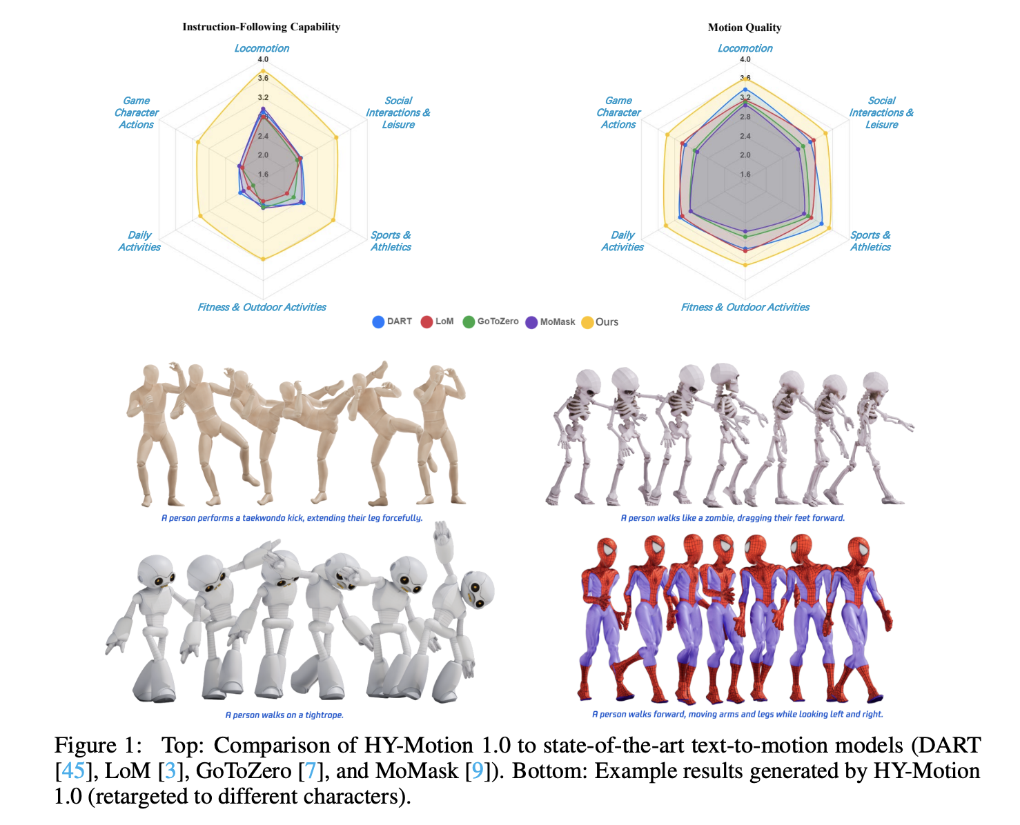
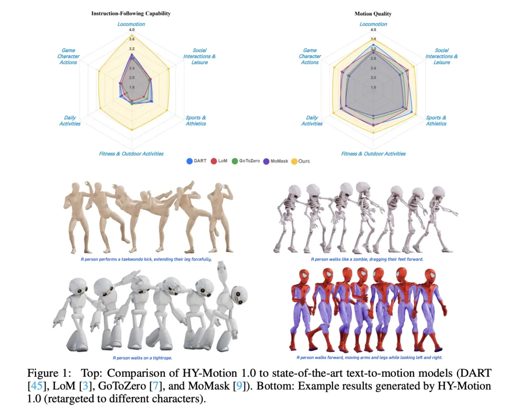
Tencent Hunyuan’s 3D Digital Human team has released HY-Motion 1.0, an open weight text-to-3D human motion generation family that scales Diffusion Transformer based Flow Matching to 1B parameters in the motion domain. The models turn natural language prompts plus an expected duration into 3D human motion clips on a unified SMPL-H skeleton and are available on GitHub and Hugging Face with code, checkpoints and a Gradio interface for local use.
HY-Motion 1.0 is a series of text-to-3D human motion generation models built on a Diffusion Transformer, DiT, trained with a Flow Matching objective. The model series showcases 2 variants, HY-Motion-1.0 with 1.0B parameters as the standard model and HY-Motion-1.0-Lite with 0.46B parameters as a lightweight option.
Both models generate skeleton based 3D character animations from simple text prompts. The output is a motion sequence on an SMPL-H skeleton that can be integrated into 3D animation or game pipelines, for example for digital humans, cinematics and interactive characters. The release includes inference scripts, a batch oriented CLI and a Gradio web app, and supports macOS, Windows and Linux.
The training data comes from 3 sources, in the wild human motion videos, motion capture data and 3D animation assets for game production. The research team starts from 12M high quality video clips from HunyuanVideo, runs shot boundary detection to split scenes and a human detector to keep clips with people, then applies the GVHMR algorithm to reconstruct SMPL X motion tracks. Motion capture sessions and 3D animation libraries contribute about 500 hours of additional motion sequences.
All data is retargeted onto a unified SMPL-H skeleton through mesh fitting and retargeting tools. A multi stage filter removes duplicate clips, abnormal poses, outliers in joint velocity, anomalous displacements, long static segments and artifacts such as foot sliding. Motions are then canonicalized, resampled to 30 fps and segmented into clips shorter than 12 seconds with a fixed world frame, Y axis up and the character facing the positive Z axis. The final corpus contains over 3,000 hours of motion, of which 400 hours are high quality 3D motion with verified captions.
On top of this, the research team defines a 3 level taxonomy. At the top level there are 6 classes, Locomotion, Sports and Athletics, Fitness and Outdoor Activities, Daily Activities, Social Interactions and Leisure and Game Character Actions. These expand into more than 200 fine grained motion categories at the leaves, which cover both simple atomic actions and concurrent or sequential motion combinations.
HY-Motion 1.0 uses the SMPL-H skeleton with 22 body joints without hands. Each frame is a 201 dimensional vector that concatenates global root translation in 3D space, global body orientation in a continuous 6D rotation representation, 21 local joint rotations in 6D form and 22 local joint positions in 3D coordinates. Velocities and foot contact labels are removed because they slowed training and did not help final quality. This representation is compatible with animation workflows and close to the DART model representation.
The core network is a hybrid HY Motion DiT. It first applies dual stream blocks that process motion latents and text tokens separately. In these blocks, each modality has its own QKV projections and MLP, and a joint attention module allows motion tokens to query semantic features from text tokens while keeping modality specific structure. The network then switches to single stream blocks that concatenate motion and text tokens into one sequence and process them with parallel spatial and channel attention modules to perform deeper multimodal fusion.
For text conditioning, the system uses a dual encoder scheme. Qwen3 8B provides token level embeddings, while a CLIP-L model provides global text features. A Bidirectional Token Refiner fixes the causal attention bias of the LLM for non autoregressive generation. These signals feed the DiT through adaptive layer normalization conditioning. Attention is asymmetric, motion tokens can attend to all text tokens, but text tokens do not attend back to motion, which prevents noisy motion states from corrupting the language representation. Temporal attention inside the motion branch uses a narrow sliding window of 121 frames, which focuses capacity on local kinematics while keeping cost manageable for long clips. Full Rotary Position Embedding is applied after concatenating text and motion tokens to encode relative positions across the whole sequence.
HY-Motion 1.0 uses Flow Matching instead of standard denoising diffusion. The model learns a velocity field along a continuous path that interpolates between Gaussian noise and real motion data. During training, the objective is a mean squared error between predicted and ground truth velocities along this path. During inference, the learned ordinary differential equation is integrated from noise to a clean trajectory, which gives stable training for long sequences and fits the DiT architecture.
A separate Duration Prediction and Prompt Rewrite module improves instruction following. It uses Qwen3 30B A3B as the base model and is trained on synthetic user style prompts generated from motion captions with a VLM and LLM pipeline, for example Gemini 2.5 Pro. This module predicts a suitable motion duration and rewrites informal prompts into normalized text that is easier for the DiT to follow. It is trained first with supervised fine tuning and then refined with Group Relative Policy Optimization, using Qwen3 235B A22B as a reward model that scores semantic consistency and duration plausibility.
Training follows a 3 stage curriculum. Stage 1 performs large scale pretraining on the full 3,000 hour dataset to learn a broad motion prior and basic text motion alignment. Stage 2 fine tunes on the 400 hour high quality set to sharpen motion detail and improve semantic correctness with a smaller learning rate. Stage 3 applies reinforcement learning, first Direct Preference Optimization using 9,228 curated human preference pairs sampled from about 40,000 generated pairs, then Flow GRPO with a composite reward. The reward combines a semantic score from a Text Motion Retrieval model and a physics score that penalizes artifacts like foot sliding and root drift, under a KL regularization term to stay close to the supervised model.
For evaluation, the team builds a test set of over 2,000 prompts that span the 6 taxonomy categories and include simple, concurrent and sequential actions. Human raters score instruction following and motion quality on a scale from 1 to 5. HY-Motion 1.0 reaches an average instruction following score of 3.24 and an SSAE score of 78.6 percent. Baseline text-to-motion systems such as DART, LoM, GoToZero and MoMask achieve scores between 2.17 and 2.31 with SSAE between 42.7 percent and 58.0 percent. For motion quality, HY-Motion 1.0 reaches 3.43 on average versus 3.11 for the best baseline.
Scaling experiments study DiT models with 0.05B, 0.46B, 0.46B trained only on 400 hours and 1B parameters. Instruction following improves steadily with model size, with the 1B model reaching an average of 3.34. Motion quality saturates around the 0.46B scale, where the 0.46B and 1B models reach similar averages between 3.26 and 3.34. Comparison of the 0.46B model trained on 3,000 hours and the 0.46B model trained only on 400 hours shows that larger data volume is key for instruction alignment, while high quality curation mainly improves realism.
Check out the and Also, feel free to follow us on and don’t forget to join our and Subscribe to . Wait! are you on telegram?
The post appeared first on .
 December 30, 2025
US support for nuclear energy is soaring. Meanwhile, coal plants are on their way out and electricity-sucking data centers are meeting huge pushback. Welcome to the next front in the energy battle.
 December 30, 2025
LLMRouter is an open source routing library from the U Lab at the University of Illinois Urbana Champaign that treats model selection as a first class system problem. It sits between applications and a pool of LLMs and chooses a model for each query based on task complexity, quality targets, and cost, all exposed through a unified Python API and CLI. The project ships with more than 16 routing models, a data generation pipeline over 11 benchmarks, and a plugin system for custom routers.
LLMRouter organizes routing algorithms into four families, Single-Round Routers, Multi-Round Routers, Personalized Routers, and Agentic Routers. Single round routers include knnrouter, svmrouter, mlprouter, mfrouter, elorouter, routerdc, automix, hybrid_llm, graphrouter, causallm_router, and the baselines smallest_llm and largest_llm. These models implement strategies such as k nearest neighbors, support vector machines, multilayer perceptrons, matrix factorization, Elo rating, dual contrastive learning, automatic model mixing, and graph based routing.
Multi round routing is exposed through router_r1, a pre trained instance of Router R1 integrated into LLMRouter. Router R1 formulates multi LLM routing and aggregation as a sequential decision process where the router itself is an LLM that alternates between internal reasoning steps and external model calls. It is trained with reinforcement learning using a rule based reward that balances format, outcome, and cost. In LLMRouter, router_r1 is available as an extra installation target with pinned dependencies tested on vllm==0.6.3 and torch==2.4.0.
Personalized routing is handled by gmtrouter, described as a graph based personalized router with user preference learning. GMTRouter represents multi turn user LLM interactions as a heterogeneous graph over users, queries, responses, and models. It runs a message passing architecture over this graph to infer user specific routing preferences from few shot interaction data, and experiments show accuracy and AUC gains over non personalized baselines.
Agentic routers in LLMRouter extend routing to multi step reasoning workflows. knnmultiroundrouter uses k nearest neighbor reasoning over multi turn traces and is intended for complex tasks. llmmultiroundrouter exposes an LLM based agentic router that performs multi step routing without its own training loop. These agentic routers share the same configuration and data formats as the other router families and can be swapped through a single CLI flag.
LLMRouter ships with a full data generation pipeline that turns standard benchmarks and LLM outputs into routing datasets. The pipeline supports 11 benchmarks, Natural QA, Trivia QA, MMLU, GPQA, MBPP, HumanEval, GSM8K, CommonsenseQA, MATH, OpenBookQA, and ARC Challenge. It runs in three explicit stages. First, data_generation.py extracts queries and ground truth labels and creates train and test JSONL splits. Second, generate_llm_embeddings.py builds embeddings for candidate LLMs from metadata. Third, api_calling_evaluation.py calls LLM APIs, evaluates responses, and fuses scores with embeddings into routing records. ()
The pipeline outputs query files, LLM embedding JSON, query embedding tensors, and routing data JSONL files. A routing entry includes fields such as task_name, query, ground_truth, metric, model_name, response, performance, embedding_id, and token_num. Configuration is handled entirely through YAML, so engineers point the scripts to new datasets and candidate model lists without modifying code.
For interactive use, llmrouter chat launches a Gradio based chat frontend over any router and configuration. The server can bind to a custom host and port and can expose a public sharing link. Query modes control how routing sees context. current_only uses only the latest user message, full_context concatenates the dialogue history, and retrieval augments the query with the top k similar historical queries. The UI visualizes model choices in real time and is driven by the same router configuration used for batch inference.
LLMRouter also provides a plugin system for custom routers. New routers live under custom_routers, subclass MetaRouter, and implement route_single and route_batch. Configuration files under that directory define data paths, hyperparameters, and optional default API endpoints. Plugin discovery scans the project custom_routers folder, a ~/.llmrouter/plugins directory, and any extra paths in the LLMROUTER_PLUGINS environment variable. Example custom routers include randomrouter, which selects a model at random, and thresholdrouter, which is a trainable router that estimates query difficulty.
knnrouter, graphrouter, routerdc, router_r1, and gmtrouter, all exposed through a unified config and CLI. router_r1 integrates the Router R1 framework, where an LLM router interleaves internal “think” steps with external “route” calls and is trained with a rule based reward that combines format, outcome, and cost to optimize performance cost trade offs.gmtrouter models users, queries, responses and LLMs as nodes in a heterogeneous graph and uses message passing to learn user specific routing preferences from few shot histories, achieving up to around 21% accuracy gains and substantial AUC improvements over strong baselines. MetaRouter that allows teams to register custom routers while reusing the same routing datasets and infrastructure.Check out the and . Also, feel free to follow us on and don’t forget to join our and Subscribe to . Wait! are you on telegram?
The post appeared first on .
December 30, 2025
In this tutorial, we build an advanced, end-to-end multi-agent research workflow using the framework. We design a coordinated society of agents, Planner, Researcher, Writer, Critic, and Finalizer, that collaboratively transform a high-level topic into a polished, evidence-grounded research brief. We securely integrate the OpenAI API, orchestrate agent interactions programmatically, and add lightweight persistent memory to retain knowledge across runs. By structuring the system around clear roles, JSON-based contracts, and iterative refinement, we demonstrate how CAMEL can be used to construct reliable, controllable, and scalable agentic pipelines. Check out the .
!pip -q install "camel-ai[all]" "python-dotenv" "rich"


import os
import json
import time
from typing import Dict, Any
from rich import print as rprint


def load_openai_key() -> str:
   key = None
   try:
       from google.colab import userdata
       key = userdata.get("OPENAI_API_KEY")
   except Exception:
       key = None
   if not key:
       import getpass
       key = getpass.getpass("Enter OPENAI_API_KEY (hidden): ").strip()
   if not key:
       raise ValueError("OPENAI_API_KEY is required.")
   return key


os.environ["OPENAI_API_KEY"] = load_openai_key()
We set up the execution environment and securely load the OpenAI API key using Colab secrets or a hidden prompt. We ensure the runtime is ready by installing dependencies and configuring authentication so the workflow can run safely without exposing credentials. Check out the .
from camel.models import ModelFactory
from camel.types import ModelPlatformType, ModelType
from camel.agents import ChatAgent
from camel.toolkits import SearchToolkit


MODEL_CFG = {"temperature": 0.2}


model = ModelFactory.create(
   model_platform=ModelPlatformType.OPENAI,
   model_type=ModelType.GPT_4O,
   model_config_dict=MODEL_CFG,
)
We initialize the CAMEL model configuration and create a shared language model instance using the ModelFactory abstraction. We standardize model behavior across all agents to ensure consistent, reproducible reasoning throughout the multi-agent pipeline. Check out the .
MEM_PATH = "camel_memory.json"


def mem_load() -> Dict[str, Any]:
   if not os.path.exists(MEM_PATH):
       return {"runs": []}
   with open(MEM_PATH, "r", encoding="utf-8") as f:
       return json.load(f)


def mem_save(mem: Dict[str, Any]) -> None:
   with open(MEM_PATH, "w", encoding="utf-8") as f:
       json.dump(mem, f, ensure_ascii=False, indent=2)


def mem_add_run(topic: str, artifacts: Dict[str, str]) -> None:
   mem = mem_load()
   mem["runs"].append({"ts": int(time.time()), "topic": topic, "artifacts": artifacts})
   mem_save(mem)


def mem_last_summaries(n: int = 3) -> str:
   mem = mem_load()
   runs = mem.get("runs", [])[-n:]
   if not runs:
       return "No past runs."
   return "n".join([f"{i+1}. topic={r['topic']} | ts={r['ts']}" for i, r in enumerate(runs)])
We implement a lightweight persistent memory layer backed by a JSON file. We store artifacts from each run and retrieve summaries of previous executions, allowing us to introduce continuity and historical context across sessions. Check out the .
def make_agent(role: str, goal: str, extra_rules: str = "") -> ChatAgent:
   system = (
       f"You are {role}.n"
       f"Goal: {goal}n"
       f"{extra_rules}n"
       "Output must be crisp, structured, and directly usable by the next agent."
   )
   return ChatAgent(model=model, system_message=system)


planner = make_agent(
   "Planner",
   "Create a compact plan and research questions with acceptance criteria.",
   "Return JSON with keys: plan, questions, acceptance_criteria."
)


researcher = make_agent(
   "Researcher",
   "Answer questions using web search results.",
   "Return JSON with keys: findings, sources, open_questions."
)


writer = make_agent(
   "Writer",
   "Draft a structured research brief.",
   "Return Markdown only."
)


critic = make_agent(
   "Critic",
   "Identify weaknesses and suggest fixes.",
   "Return JSON with keys: issues, fixes, rewrite_instructions."
)


finalizer = make_agent(
   "Finalizer",
   "Produce the final improved brief.",
   "Return Markdown only."
)


search_tool = SearchToolkit().search_duckduckgo
researcher = ChatAgent(
   model=model,
   system_message=researcher.system_message,
   tools=[search_tool],
)
We define the core agent roles and their responsibilities within the workflow. We construct specialized agents with clear goals and output contracts, and we enhance the Researcher by attaching a web search tool for evidence-grounded responses. Check out the .
def step_json(agent: ChatAgent, prompt: str) -> Dict[str, Any]:
   res = agent.step(prompt)
   txt = res.msgs[0].content.strip()
   try:
       return json.loads(txt)
   except Exception:
       return {"raw": txt}


def step_text(agent: ChatAgent, prompt: str) -> str:
   res = agent.step(prompt)
   return res.msgs[0].content
We abstract interaction patterns with agents into helper functions that enforce structured JSON or free-text outputs. We simplify orchestration by handling parsing and fallback logic centrally, making the pipeline more robust to formatting variability. Check out the .
def run_workflow(topic: str) -> Dict[str, str]:
   rprint(mem_last_summaries(3))


   plan = step_json(
       planner,
       f"Topic: {topic}nCreate a tight plan and research questions."
   )


   research = step_json(
       researcher,
       f"Research the topic using web search.n{json.dumps(plan)}"
   )


   draft = step_text(
       writer,
       f"Write a research brief using:n{json.dumps(research)}"
   )


   critique = step_json(
       critic,
       f"Critique the draft:n{draft}"
   )


   final = step_text(
       finalizer,
       f"Rewrite using critique:n{json.dumps(critique)}nDraft:n{draft}"
   )


   artifacts = {
       "plan_json": json.dumps(plan, indent=2),
       "research_json": json.dumps(research, indent=2),
       "draft_md": draft,
       "critique_json": json.dumps(critique, indent=2),
       "final_md": final,
   }


   mem_add_run(topic, artifacts)
   return artifacts


TOPIC = "Agentic multi-agent research workflow with quality control"
artifacts = run_workflow(TOPIC)
print(artifacts["final_md"])
We orchestrate the complete multi-agent workflow from planning to finalization. We sequentially pass artifacts between agents, apply critique-driven refinement, persist results to memory, and produce a finalized research brief ready for downstream use.
In conclusion, we implemented a practical CAMEL-based multi-agent system that mirrors real-world research and review workflows. We showed how clearly defined agent roles, tool-augmented reasoning, and critique-driven refinement lead to higher-quality outputs while reducing hallucinations and structural weaknesses. We also established a foundation for extensibility by persisting artifacts and enabling reuse across sessions. This approach allows us to move beyond single-prompt interactions and toward robust agentic systems that can be adapted for research, analysis, reporting, and decision-support tasks at scale.
Check out the . Also, feel free to follow us on and don’t forget to join our and Subscribe to . Wait! are you on telegram?
The post appeared first on .
 December 29, 2025
Google’s AI is now even smarter, and more versatile.
December 29, 2025
In this tutorial, we demonstrate how to design a contract-first agentic decision system using , treating structured schemas as non-negotiable governance contracts rather than optional output formats. We show how we define a strict decision model that encodes policy compliance, risk assessment, confidence calibration, and actionable next steps directly into the agent’s output schema. By combining Pydantic validators with PydanticAI’s retry and self-correction mechanisms, we ensure that the agent cannot produce logically inconsistent or non-compliant decisions. Throughout the workflow, we focus on building an enterprise-grade decision agent that reasons under constraints, making it suitable for real-world risk, compliance, and governance scenarios rather than toy prompt-based demos. Check out the .
!pip -q install -U pydantic-ai pydantic openai nest_asyncio


import os
import time
import asyncio
import getpass
from dataclasses import dataclass
from typing import List, Literal


import nest_asyncio
nest_asyncio.apply()


from pydantic import BaseModel, Field, field_validator
from pydantic_ai import Agent
from pydantic_ai.models.openai import OpenAIChatModel
from pydantic_ai.providers.openai import OpenAIProvider


OPENAI_API_KEY = os.getenv("OPENAI_API_KEY")
if not OPENAI_API_KEY:
   try:
       from google.colab import userdata
       OPENAI_API_KEY = userdata.get("OPENAI_API_KEY")
   except Exception:
       OPENAI_API_KEY = None
if not OPENAI_API_KEY:
   OPENAI_API_KEY = getpass.getpass("Enter OPENAI_API_KEY: ").strip()
We set up the execution environment by installing the required libraries and configuring asynchronous execution for Google Colab. We securely load the OpenAI API key and ensure the runtime is ready to handle async agent calls. This establishes a stable foundation for running the contract-first agent without environment-related issues. Check out the .
class RiskItem(BaseModel):
   risk: str = Field(..., min_length=8)
   severity: Literal["low", "medium", "high"]
   mitigation: str = Field(..., min_length=12)


class DecisionOutput(BaseModel):
   decision: Literal["approve", "approve_with_conditions", "reject"]
   confidence: float = Field(..., ge=0.0, le=1.0)
   rationale: str = Field(..., min_length=80)
   identified_risks: List[RiskItem] = Field(..., min_length=2)
   compliance_passed: bool
   conditions: List[str] = Field(default_factory=list)
   next_steps: List[str] = Field(..., min_length=3)
   timestamp_unix: int = Field(default_factory=lambda: int(time.time()))


   @field_validator("confidence")
   @classmethod
   def confidence_vs_risk(cls, v, info):
       risks = info.data.get("identified_risks") or []
       if any(r.severity == "high" for r in risks) and v > 0.70:
           raise ValueError("confidence too high given high-severity risks")
       return v


   @field_validator("decision")
   @classmethod
   def reject_if_non_compliant(cls, v, info):
       if info.data.get("compliance_passed") is False and v != "reject":
           raise ValueError("non-compliant decisions must be reject")
       return v


   @field_validator("conditions")
   @classmethod
   def conditions_required_for_conditional_approval(cls, v, info):
       d = info.data.get("decision")
       if d == "approve_with_conditions" and (not v or len(v) < 2):
           raise ValueError("approve_with_conditions requires at least 2 conditions")
       if d == "approve" and v:
           raise ValueError("approve must not include conditions")
       return v
We define the core decision contract using strict Pydantic models that precisely describe a valid decision. We encode logical constraints such as confidence–risk alignment, compliance-driven rejection, and conditional approvals directly into the schema. This ensures that any agent output must satisfy business logic, not just syntactic structure. Check out the .
@dataclass
class DecisionContext:
   company_policy: str
   risk_threshold: float = 0.6


model = OpenAIChatModel(
   "gpt-5",
   provider=OpenAIProvider(api_key=OPENAI_API_KEY),
)


agent = Agent(
   model=model,
   deps_type=DecisionContext,
   output_type=DecisionOutput,
   system_prompt="""
You are a corporate decision analysis agent.
You must evaluate risk, compliance, and uncertainty.
All outputs must strictly satisfy the DecisionOutput schema.
"""
)
We inject enterprise context through a typed dependency object and initialize the OpenAI-backed PydanticAI agent. We configure the agent to produce only structured decision outputs that conform to the predefined contract. This step formalizes the separation between business context and model reasoning. Check out the .
@agent.output_validator
def ensure_risk_quality(result: DecisionOutput) -> DecisionOutput:
   if len(result.identified_risks) < 2:
       raise ValueError("minimum two risks required")
   if not any(r.severity in ("medium", "high") for r in result.identified_risks):
       raise ValueError("at least one medium or high risk required")
   return result


@agent.output_validator
def enforce_policy_controls(result: DecisionOutput) -> DecisionOutput:
   policy = CURRENT_DEPS.company_policy.lower()
   text = (
       result.rationale
       + " ".join(result.next_steps)
       + " ".join(result.conditions)
   ).lower()
   if result.compliance_passed:
       if not any(k in text for k in ["encryption", "audit", "logging", "access control", "key management"]):
           raise ValueError("missing concrete security controls")
   return result
We add output validators that act as governance checkpoints after the model generates a response. We force the agent to identify meaningful risks and to explicitly reference concrete security controls when claiming compliance. If these constraints are violated, we trigger automatic retries to enforce self-correction. Check out the .
async def run_decision():
   global CURRENT_DEPS
   CURRENT_DEPS = DecisionContext(
       company_policy=(
           "No deployment of systems handling personal data or transaction metadata "
           "without encryption, audit logging, and least-privilege access control."
       )
   )


   prompt = """
Decision request:
Deploy an AI-powered customer analytics dashboard using a third-party cloud vendor.
The system processes user behavior and transaction metadata.
Audit logging is not implemented and customer-managed keys are uncertain.
"""


   result = await agent.run(prompt, deps=CURRENT_DEPS)
   return result.output


decision = asyncio.run(run_decision())


from pprint import pprint
pprint(decision.model_dump())
We run the agent on a realistic decision request and capture the validated structured output. We demonstrate how the agent evaluates risk, policy compliance, and confidence before producing a final decision. This completes the end-to-end contract-first decision workflow in a production-style setup.
In conclusion, we demonstrate how to move from free-form LLM outputs to governed, reliable decision systems using PydanticAI. We show that by enforcing hard contracts at the schema level, we can automatically align decisions with policy requirements, risk severity, and confidence realism without manual prompt tuning. This approach allows us to build agents that fail safely, self-correct when constraints are violated, and produce auditable, structured outputs that downstream systems can trust. Ultimately, we demonstrate that contract-first agent design enables us to deploy agentic AI as a dependable decision layer within production and enterprise environments.
Check out the . Also, feel free to follow us on and don’t forget to join our and Subscribe to . Wait! are you on telegram?
The post appeared first on .
 December 28, 2025
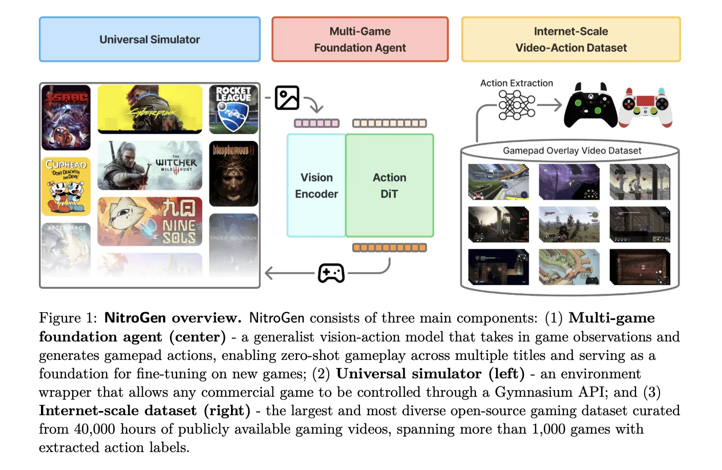
NVIDIA AI research team released NitroGen, an open vision action foundation model for generalist gaming agents that learns to play commercial games directly from pixels and gamepad actions using internet video at scale. NitroGen is trained on 40,000 hours of gameplay across more than 1,000 games and comes with an open dataset, a universal simulator, and a pre trained policy.
The NitroGen pipeline starts from publicly available gameplay videos that include input overlays, for example gamepad visualizations that streamers place in a corner of the screen. The research team collects 71,000 hours of raw video with such overlays, then applies quality filtering based on action density, which leaves 55% of the data, about 40,000 hours, spanning more than 1,000 games.
The curated dataset contains 38,739 videos from 818 creators. The distribution covers a wide range of titles. There are 846 games with more than 1 hour of data, 91 games with more than 100 hours, and 15 games with more than 1,000 hours each. Action RPGs account for 34.9 percent of the hours, platformers for 18.4 percent, and action adventure titles for 9.2 percent, with the rest spread across sports, roguelike, racing and other genres.
To recover frame level actions from raw streams, NitroGen uses a three stage action extraction pipeline. First, a template matching module localizes the controller overlay using about 300 controller templates. For each video, the system samples 25 frames and matches SIFT and XFeat features between frames and templates, then estimates an affine transform when at least 20 inliers support a match. This yields a crop of the controller region for all frames.
Second, a SegFormer based hybrid classification segmentation model parses the controller crops. The model takes two consecutive frames concatenated spatially and outputs joystick locations on an 11 by 11 grid plus binary button states. It is trained on 8 million synthetic images rendered with different controller templates, opacities, sizes and compression settings, using AdamW with learning rate 0.0001, weight decay 0.1, and batch size 256.
Third, the pipeline refines joystick positions and filters low activity segments. Joystick coordinates are normalized to the range from −1.0 to 1.0 using the 99th percentile of absolute x and y values to reduce outliers. Chunks where fewer than 50 percent of timesteps have non zero actions are removed, which avoids over predicting the null action during policy training.
A separate benchmark with ground truth controller logs shows that joystick predictions reach an average R² of 0.84 and button frame accuracy reaches 0.96 across major controller families such as Xbox and PlayStation. This validates that automatic annotations are accurate enough for large scale behavior cloning.
NitroGen includes a universal simulator that wraps commercial Windows games in a Gymnasium compatible interface. The wrapper intercepts the game engine system clock to control simulation time and supports frame by frame interaction without modifying game code, for any title that uses the system clock for physics and interactions.
Observations in this benchmark are single RGB frames. Actions are defined as a unified controller space with a 16 dimensional binary vector for gamepad buttons, four d pad buttons, four face buttons, two shoulders, two triggers, two joystick thumb buttons, start and back, plus a 4 dimensional continuous vector for joystick positions, left and right x,y. This unified layout allows direct transfer of one policy across many games.
The evaluation suite covers 10 commercial games and 30 tasks. There are 5 two dimensional games, three side scrollers and two top down roguelikes, and 5 three dimensional games, two open world games, two combat focused action RPGs and one sports title. Tasks fall into 11 combat tasks, 10 navigation tasks, and 9 game specific tasks with custom objectives.
The NitroGen foundation policy follows the GR00T N1 architecture pattern for embodied agents. It discards the language and state encoders, and keeps a vision encoder plus a single action head. Input is one RGB frame at 256 by 256 resolution. A SigLIP 2 vision transformer encodes this frame into 256 image tokens.
A diffusion transformer, DiT, generates 16 step chunks of future actions. During training, noisy action chunks are embedded by a multilayer perceptron into action tokens, processed by a stack of DiT blocks with self attention and cross attention to visual tokens, then decoded back into continuous action vectors. The training objective is conditional flow matching with 16 denoising steps over each 16 action chunk.
The released checkpoint has 4.93 × 10^8 parameters. The model card describes the output as a 21 by 16 tensor, where 17 dimensions correspond to binary button states and 4 dimensions store two two dimensional joystick vectors, over 16 future timesteps. This representation is consistent with the unified action space, up to reshaping of the joystick components.
NitroGen is trained purely with large scale behavior cloning on the internet video dataset. There is no reinforcement learning and no reward design in the base model. Image augmentations include random brightness, contrast, saturation, hue, small rotations, and random crops. Training uses AdamW with weight decay 0.001, a warmup stable decay learning rate schedule with constant phase at 0.0001, and an exponential moving average of weights with decay 0.9999.
After pre training on the full dataset, NitroGen 500M already achieves non trivial task completion rates in zero shot evaluation across all games in the benchmark. Average completion rates stay in the range from about 45 percent to 60 percent across combat, navigation and game specific tasks, and across two dimensional and three dimensional games, despite the noise in internet supervision.
For transfer to unseen games, the research team hold out a title, pre train on the remaining data, and then fine tune on the held out game under a fixed data and compute budget. On an isometric roguelike, fine tuning from NitroGen gives an average relative improvement of about 10 percent compared with training from scratch. On a three dimensional action RPG, the average gain is about 25 percent, and for some combat tasks in the low data regime, 30 hours, the relative improvement reaches 52 percent.
Check out the and . Also, feel free to follow us on and don’t forget to join our and Subscribe to . Wait! are you on telegram?
The post appeared first on .
 December 28, 2025
The battle for AI dominance has left a large footprint—and it’s only getting bigger and more expensive.