AI in web design

In this tutorial, we build an advanced, fully autonomous logistics simulation in which multiple smart delivery trucks operate within a dynamic city-wide road network. We design the system so that each truck behaves as an agent capable of bidding on delivery orders, planning optimal routes, managing battery levels, seeking charging stations, and maximizing profit through self-interested decision-making. Through each code snippet, we explore how agentic behaviors emerge from simple rules, how competition shapes order allocation, and how a graph-based world enables realistic movement, routing, and resource constraints. Check out the .

import networkx as nx
import matplotlib.pyplot as plt
import random
import time
from IPython.display import clear_output
from dataclasses import dataclass, field
from typing import List, Dict, Optional


NUM_NODES = 30
CONNECTION_RADIUS = 0.25
NUM_AGENTS = 5
STARTING_BALANCE = 1000
FUEL_PRICE = 2.0
PAYOUT_MULTIPLIER = 5.0
BATTERY_CAPACITY = 100
CRITICAL_BATTERY = 25


@dataclass
class Order:
   id: str
   target_node: int
   weight_kg: int
   payout: float
   status: str = "pending"


class AgenticTruck:
   def __init__(self, agent_id, start_node, graph, capacity=100):
       self.id = agent_id
       self.current_node = start_node
       self.graph = graph
       self.battery = BATTERY_CAPACITY
       self.balance = STARTING_BALANCE
       self.capacity = capacity
       self.state = "IDLE"
       self.path: List[int] = []
       self.current_order: Optional[Order] = None
       self.target_node: int = start_node

We set up all the core building blocks of the simulation, including imports, global parameters, and the basic data structures. We also define the AgenticTruck class and initialize key attributes, including position, battery, balance, and operating state. We lay the foundation for all agent behaviors to evolve. Check out the .

 def get_path_cost(self, start, end):
       try:
           length = nx.shortest_path_length(self.graph, start, end, weight='weight')
           path = nx.shortest_path(self.graph, start, end, weight='weight')
           return length, path
       except nx.NetworkXNoPath:
           return float('inf'), []


   def find_nearest_charger(self):
       chargers = [n for n, attr in self.graph.nodes(data=True) if attr.get('type') == 'charger']
       best_charger = None
       min_dist = float('inf')
       best_path = []
       for charger in chargers:
           dist, path = self.get_path_cost(self.current_node, charger)
           if dist < min_dist:
               min_dist = dist
               best_charger = charger
               best_path = path
       return best_charger, best_path


   def calculate_bid(self, order):
       if order.weight_kg > self.capacity:
           return float('inf')
       if self.state != "IDLE" or self.battery < CRITICAL_BATTERY:
           return float('inf')
       dist_to_target, _ = self.get_path_cost(self.current_node, order.target_node)
       fuel_cost = dist_to_target * FUEL_PRICE
       expected_profit = order.payout - fuel_cost
       if expected_profit < 10:
           return float('inf')
       return dist_to_target


   def assign_order(self, order):
       self.current_order = order
       self.state = "MOVING"
       self.target_node = order.target_node
       _, self.path = self.get_path_cost(self.current_node, self.target_node)
       if self.path: self.path.pop(0)


   def go_charge(self):
       charger_node, path = self.find_nearest_charger()
       if charger_node is not None:
           self.state = "TO_CHARGER"
           self.target_node = charger_node
           self.path = path
           if self.path: self.path.pop(0)

We implement advanced decision-making logic for the trucks. We calculate shortest paths, identify nearby charging stations, and evaluate whether an order is profitable and feasible. We also prepare the truck to accept assignments or proactively seek charging when needed. Check out the .

 def step(self):
       if self.state == "IDLE" and self.battery < CRITICAL_BATTERY:
           self.go_charge()


       if self.state == "CHARGING":
           self.battery += 10
           self.balance -= 5
           if self.battery >= 100:
               self.battery = 100
               self.state = "IDLE"
           return


       if self.path:
           next_node = self.path[0]
           edge_data = self.graph.get_edge_data(self.current_node, next_node)
           distance = edge_data['weight']
           self.current_node = next_node
           self.path.pop(0)
           self.battery -= (distance * 2)
           self.balance -= (distance * FUEL_PRICE)


           if not self.path:
               if self.state == "MOVING":
                   self.balance += self.current_order.payout
                   self.current_order.status = "completed"
                   self.current_order = None
                   self.state = "IDLE"
               elif self.state == "TO_CHARGER":
                   self.state = "CHARGING"

We manage the step-by-step actions of each truck as the simulation runs. We handle battery recharging, financial impacts of movement, fuel consumption, and order completion. We ensure that agents transition smoothly between states, such as moving, charging, and idling. Check out the .

class Simulation:
   def __init__(self):
       self.setup_graph()
       self.setup_agents()
       self.orders = []
       self.order_count = 0


   def setup_graph(self):
       self.G = nx.random_geometric_graph(NUM_NODES, CONNECTION_RADIUS)
       for (u, v) in self.G.edges():
           self.G.edges[u, v]['weight'] = random.uniform(1.0, 3.0)
       for i in self.G.nodes():
           r = random.random()
           if r < 0.15:
               self.G.nodes[i]['type'] = 'charger'
               self.G.nodes[i]['color'] = 'red'
           else:
               self.G.nodes[i]['type'] = 'house'
               self.G.nodes[i]['color'] = '#A0CBE2'


   def setup_agents(self):
       self.agents = []
       for i in range(NUM_AGENTS):
           start_node = random.randint(0, NUM_NODES-1)
           cap = random.choice([50, 100, 200])
           self.agents.append(AgenticTruck(i, start_node, self.G, capacity=cap))


   def generate_order(self):
       target = random.randint(0, NUM_NODES-1)
       weight = random.randint(10, 120)
       payout = random.randint(50, 200)
       order = Order(id=f"ORD-{self.order_count}", target_node=target, weight_kg=weight, payout=payout)
       self.orders.append(order)
       self.order_count += 1
       return order


   def run_market(self):
       for order in self.orders:
           if order.status == "pending":
               bids = {agent: agent.calculate_bid(order) for agent in self.agents}
               valid_bids = {k: v for k, v in bids.items() if v != float('inf')}
               if valid_bids:
                   winner = min(valid_bids, key=valid_bids.get)
                   winner.assign_order(order)
                   order.status = "assigned"

We create the simulated world and orchestrate agent interactions. We generate the graph-based city, spawn trucks with varying capacities, and produce new delivery orders. We also implement a simple market where agents bid for tasks based on profitability and distance. Check out the .

  def step(self):
       if random.random() < 0.3:
           self.generate_order()
       self.run_market()
       for agent in self.agents:
           agent.step()


   def visualize(self, step_num):
       clear_output(wait=True)
       plt.figure(figsize=(10, 8))
       pos = nx.get_node_attributes(self.G, 'pos')
       node_colors = [self.G.nodes[n]['color'] for n in self.G.nodes()]
       nx.draw(self.G, pos, node_color=node_colors, with_labels=True, node_size=300, edge_color='gray', alpha=0.6)


       for agent in self.agents:
           x, y = pos[agent.current_node]
           jitter_x = x + random.uniform(-0.02, 0.02)
           jitter_y = y + random.uniform(-0.02, 0.02)
           color = 'green' if agent.state == "IDLE" else ('orange' if agent.state == "MOVING" else 'red')
           plt.plot(jitter_x, jitter_y, marker='s', markersize=12, color=color, markeredgecolor='black')
           plt.text(jitter_x, jitter_y+0.03, f"A{agent.id}n${int(agent.balance)}n{int(agent.battery)}%",
                    fontsize=8, ha='center', fontweight='bold', bbox=dict(facecolor='white', alpha=0.7, pad=1))


       for order in self.orders:
           if order.status in ["assigned", "pending"]:
               ox, oy = pos[order.target_node]
               plt.plot(ox, oy, marker='*', markersize=15, color='gold', markeredgecolor='black')


       plt.title(f"Graph-Based Logistics Swarm | Step: {step_num}nRed Nodes = Chargers | Gold Stars = Orders", fontsize=14)
       plt.show()




print("Initializing Advanced Simulation...")
sim = Simulation()


for t in range(60):
   sim.step()
   sim.visualize(t)
   time.sleep(0.5)


print("Simulation Finished.")

We step through the full simulation loop and visualize the logistics swarm in real time. We update agent states, draw the network, display active orders, and animate each truck’s movement. By running this loop, we observe the emergent coordination and competition that define our multi-agent logistics ecosystem.

In conclusion, we saw how the individual components, graph generation, autonomous routing, battery management, auctions, and visualization, come together to form a living, evolving system of agentic trucks. We watch as agents negotiate workloads, compete for profitable opportunities, and respond to environmental pressures such as distance, fuel costs, and charging needs. By running the simulation, we observe emergent dynamics that mirror real-world fleet behavior, providing a powerful sandbox for experimenting with logistics intelligence.

Check out the . Also, feel free to follow us on  and don’t forget to join our  and Subscribe to . Wait! are you on telegram? 

The post appeared first on .

Agentic AI systems sit on top of large language models and connect to tools, memory, and external environments. They already support scientific discovery, software development, and clinical research, yet they still struggle with unreliable tool use, weak long horizon planning, and poor generalization. The latest research paper ‘Adaptation of Agentic AI‘ from Stanford, Harvard, UC Berkeley, Caltech proposes a unified view of how these systems should adapt and maps existing methods into a compact, mathematically defined framework.

How this research paper models an agentic AI system?

The research survey models an agentic AI system as a foundation model agent along with 3 key components. A planning module decomposes goals into sequences of actions, using static procedures such as Chain-of-Thought and Tree-of-Thought, or dynamic procedures such as ReAct and Reflexion that react to feedback. A tool use module connects the agent to web search engines, APIs, code execution environments, Model Context Protocols, and browser automation. A memory module stores short term context and long term knowledge, accessed through retrieval augmented generation. Adaptation changes prompts or parameters for these components using supervised fine tuning, preference based methods such as Direct Preference Optimization, reinforcement learning methods such as Proximal Policy Optimization and Group Relative Policy Optimization, and parameter efficient techniques such as low rank adaptation.

Four adaptation paradigms

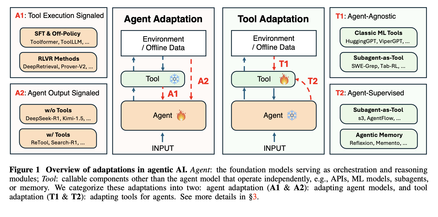
The framework defines 4 adaptation paradigms by combining 2 binary choices. The first dimension is the target, agent adaptation versus tool adaptation. The second dimension is the supervision signal, tool execution versus agent output. This yields A1 and A2 for adapting the agent, and T1 and T2 for adapting tools.

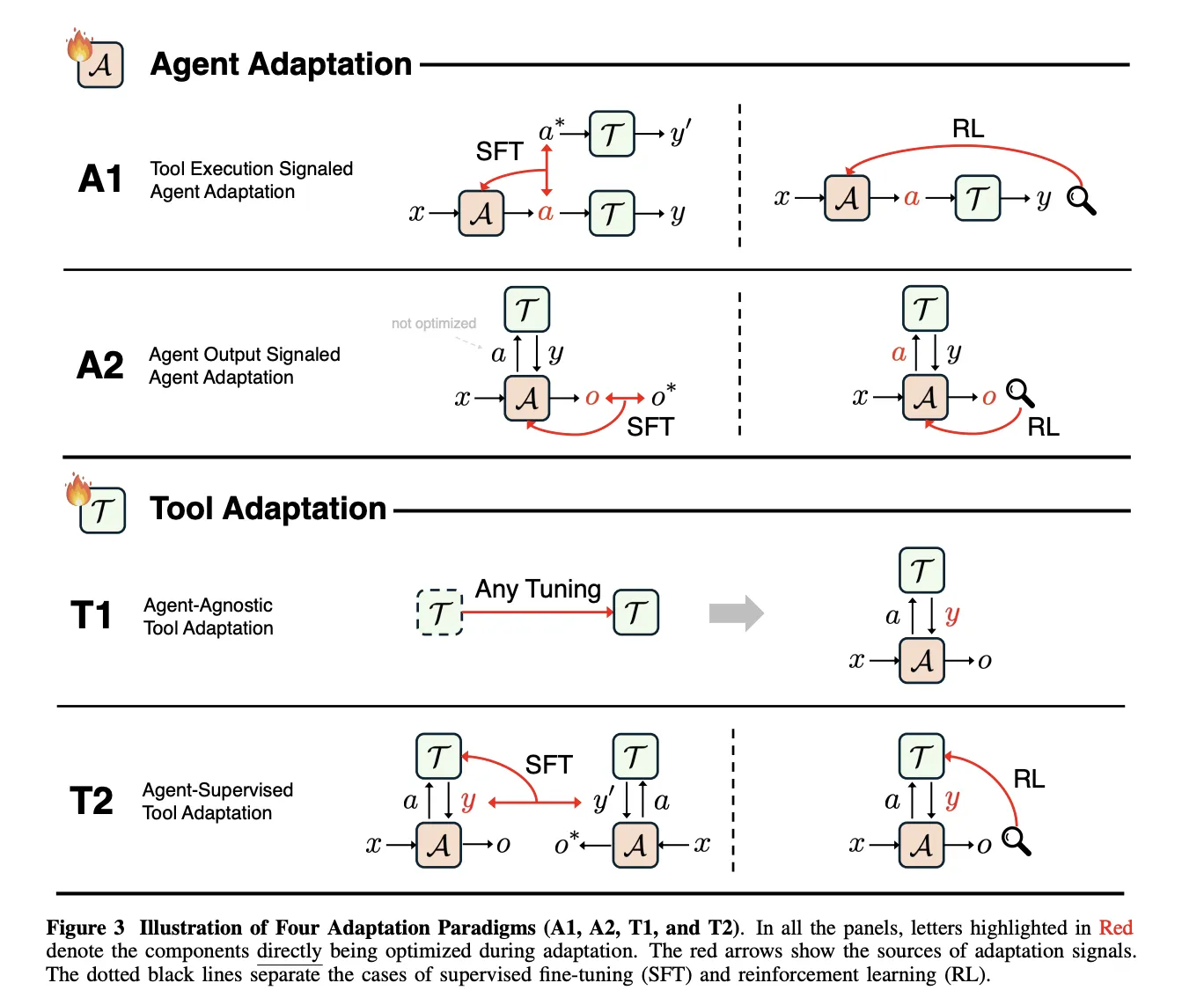
A1, Tool Execution Signaled Agent Adaptation, optimizes the agent using feedback derived from tool execution. A2, Agent Output Signaled Agent Adaptation, optimizes the agent using a signal defined only on its final outputs. T1, Agent-Agnostic Tool Adaptation, optimizes tools without referring to a particular agent. T2, Agent-Supervised Tool Adaptation, optimizes tools under supervision from a fixed agent.

A1, learning from verifiable tool feedback

In A1, the agent receives an input x, produces a structured tool call a, the tools return a result y, and the learning objective O_tool measures tool success, for example execution correctness or retrieval quality. The paper covers both supervised imitation of successful tool trajectories and reinforcement learning that uses verifiable tool outcomes as reward.

Toolformer, ToolAlpaca, and Gorilla illustrate supervised A1 methods, since each uses execution results of real tools to construct or filter training traces before imitation. All of them keep the supervision signal defined at the tool behavior level, not at the final answer level.

DeepRetrieval is a central A1 reinforcement learning example. It frames query reformulation as a Markov decision process where the state is the user query, the action is a rewritten query, and the reward combines retrieval metrics such as Recall and nDCG, a format term, and, for text to SQL, SQL execution accuracy. The policy is trained with KL regularized Proximal Policy Optimization and the same objective covers literature search, corpus question answering, and text to SQL.

A2, learning from final agent outputs

A2 covers cases where the optimization objective O_agent depends only on the final output o produced by the agent, even when the agent uses tools internally. The survey shows that supervising only o is not enough to teach tools, because the agent can ignore tools and still improve likelihood. Effective A2 systems therefore combine supervision on tool calls with supervision on final answers, or assign sparse rewards such as exact match accuracy to o and propagate them back through the full trajectory.

T1, agent agnostic tool training

T1 freezes the main agent and optimizes tools so that they are broadly reusable. The objective O_tool depends only on tool outputs and is measured by metrics such as retrieval accuracy, ranking quality, simulation fidelity, or downstream task success. A1 trained search policies, such as DeepRetrieval, can later be reused as T1 tools inside new agentic systems without modifying the main agent.

T2, tools optimized under a frozen agent

T2 assumes a powerful but fixed agent A, which is common when the agent is a closed source foundation model. The tool executes calls and returns results that the agent then uses to produce o. The optimization objective again lives on O_agent, but the trainable parameters belong to the tool. The paper describes quality weighted training, target based training, and reinforcement learning variants that all derive learning signals for the tool from the final agent outputs.

The survey treats long term memory as a special case of T2. Memory is an external store written and read through learned functions, and the agent remains frozen. Recent T2 systems include s3, which trains a 7 billion parameter searcher that maximizes a Gain Beyond RAG reward defined by a frozen generator, and AgentFlow, which trains a planner to orchestrate mostly frozen Qwen2.5 based modules using Flow GRPO.

Key Takeaways

• The research defines a precise 4 paradigm framework for adapting agentic AI by crossing 2 dimensions, whether adaptation targets the agent or tools, and whether the supervision signal comes from tool execution or from final agent outputs.
• A1 methods such as Toolformer, ToolAlpaca, Gorilla, and DeepRetrieval adapt the agent directly from verifiable tool feedback, including retrieval metrics, SQL execution accuracy, and code execution results, often optimized with KL regularized Proximal Policy Optimization.
• A2 methods optimize the agent from signals on final outputs, for example answer accuracy, and the paper shows that systems must still supervise tool calls or propagate sparse rewards through full trajectories, otherwise the agent can ignore tools while still improving likelihood.
• T1 and T2 shift learning to tools and memory, T1 trains generally useful retrievers, searchers, and simulators without a specific agent in mind, while T2 adapts tools under a frozen agent, as in s3 and AgentFlow where a fixed generator supervises a learned searcher and planner.
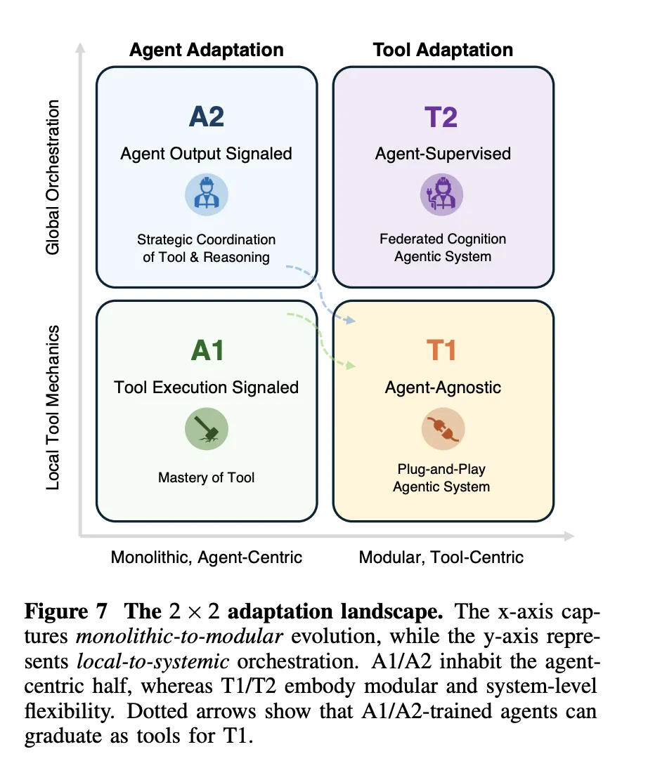
• The research team introduce an adaptation landscape that relates monolithic versus modular and local versus systemic control, and they argue that practical systems will combine rare A1 or A2 updates on a strong base model with frequent T1 and T2 adaptation of retrievers, search policies, simulators, and memory for robustness and scalability.

Check out the  and . Also, feel free to follow us on  and don’t forget to join our  and Subscribe to . Wait! are you on telegram? 

The post appeared first on .

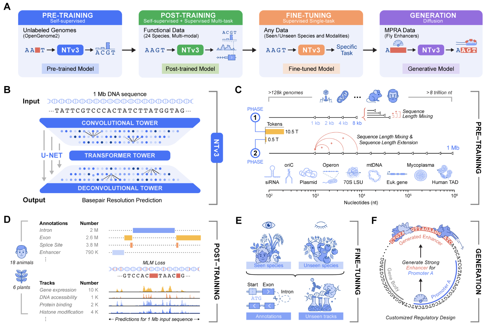
Genomic prediction and design now require models that connect local motifs with megabase scale regulatory context and that operate across many organisms. Nucleotide Transformer v3, or NTv3, is InstaDeep’s new multi species genomics foundation model for this setting. It unifies representation learning, functional track and genome annotation prediction, and controllable sequence generation in a single backbone that runs on 1 Mb contexts at single nucleotide resolution.

Earlier Nucleotide Transformer models already showed that self supervised pretraining on thousands of genomes yields strong features for molecular phenotype prediction. The original series included models from 50M to 2.5B parameters trained on 3,200 human genomes and 850 additional genomes from diverse species. NTv3 keeps this sequence only pretraining idea but extends it to longer contexts and adds explicit functional supervision and a generative mode.

Architecture for 1 Mb genomic windows

NTv3 uses a U-Net style architecture that targets very long genomic windows. A convolutional downsampling tower compresses the input sequence, a transformer stack models long range dependencies in that compressed space, and a deconvolution tower restores base level resolution for prediction and generation. Inputs are tokenized at the character level over A, T, C, G, N with special tokens such as <unk>, <pad>, <mask>, <cls>, <eos>, and <bos>. Sequence length must be a multiple of 128 tokens, and the reference implementation uses padding to enforce this constraint. All public checkpoints use single base tokenization with a vocabulary size of 11 tokens.

The smallest public model, NTv3 8M pre, has about 7.69M parameters with hidden dimension 256, FFN dimension 1,024, 2 transformer layers, 8 attention heads, and 7 downsample stages. At the high end, NTv3 650M uses hidden dimension 1,536, FFN dimension 6,144, 12 transformer layers, 24 attention heads, and 7 downsample stages, and adds conditioning layers for species specific prediction heads.

Training data

The NTv3 model is pretrained on 9 trillion base pairs from the OpenGenome2 resource using base resolution masked language modeling. After this stage, the model is post trained with a joint objective that integrates continued self supervision with supervised learning on approximately 16,000 functional tracks and annotation labels from 24 animal and plant species.

Performance and Ntv3 Benchmark

After post training NTv3 achieves state of the art accuracy for functional track prediction and genome annotation across species. It outperforms strong sequence to function models and previous genomic foundation models on existing public benchmarks and on the new Ntv3 Benchmark, which is defined as a controlled downstream fine tuning suite with standardized 32 kb input windows and base resolution outputs.

The Ntv3 Benchmark currently consists of 106 long range, single nucleotide, cross assay, cross species tasks. Because NTv3 sees thousands of tracks across 24 species during post training, the model learns a shared regulatory grammar that transfers between organisms and assays and supports coherent long range genome to function inference.

From prediction to controllable sequence generation

Beyond prediction, NTv3 can be fine tuned into a controllable generative model via masked diffusion language modeling. In this mode the model receives conditioning signals that encode desired enhancer activity levels and promoter selectivity, and it fills masked spans in the DNA sequence in a way that is consistent with those conditions.

In experiments described in the launch materials, the team designs 1,000 enhancer sequences with specified activity and promoter specificity and validates them in vitro using STARR seq assays in collaboration with the Stark Lab. The results show that these generated enhancers recover the intended ordering of activity levels and reach more than 2 times improved promoter specificity compared with baselines.

Key Takeaways

1. NTv3 is a long range, multi species genomics foundation model: It unifies representation learning, functional track prediction, genome annotation, and controllable sequence generation in a single U Net style architecture that supports 1 Mb nucleotide resolution context across 24 animal and plant species.
2. The model is trained on 9 trillion base pairs with joint self supervised and supervised objectives: NTv3 is pretrained on 9 trillion base pairs from OpenGenome2 with base resolution masked language modeling, then post trained on more than 16,000 functional tracks and annotation labels from 24 species using a joint objective that mixes continued self supervision with supervised learning.
3. NTv3 achieves state of the art performance on the Ntv3 Benchmark: After post training, NTv3 reaches state of the art accuracy for functional track prediction and genome annotation across species and outperforms previous sequence to function models and genomics foundation models on public benchmarks and on the Ntv3 Benchmark, which contains 106 standardized long range downstream tasks with 32 kb input and base resolution outputs.
4. The same backbone supports controllable enhancer design validated with STARR seq: NTv3 can be fine tuned as a controllable generative model using masked diffusion language modeling to design enhancer sequences with specified activity levels and promoter selectivity, and these designs are validated experimentally with STARR seq assays that confirm the intended activity ordering and improved promoter specificity.

Check out the ,  and . Also, feel free to follow us on  and don’t forget to join our  and Subscribe to . Wait! are you on telegram? 

The post appeared first on .

Google Health AI team has released MedASR, an open weights medical speech to text model that targets clinical dictation and physician patient conversations and is designed to plug directly into modern AI workflows.

What MedASR is and where it fits?

MedASR is a speech to text model based on the Conformer architecture and is pre trained for medical dictation and transcription. It is positioned as a starting point for developers who want to build healthcare based voice applications such as radiology dictation tools or visit note capture systems.

The model has 105 million parameters and accepts mono channel audio at 16000 hertz with 16 bit integer waveforms. It produces text only output, so it drops directly into downstream natural language processing or generative models such as MedGemma.

MedASR sits inside the Health AI Developer Foundations portfolio, alongside MedGemma, MedSigLIP and other domain specific medical models that share common terms of use and a consistent governance story.

Training data and domain specialization

MedASR is trained on a diverse corpus of de identified medical speech. The dataset includes about 5000 hours of physician dictations and clinical conversations across radiology, internal medicine and family medicine.

The training pairs audio segments with transcripts and metadata. Subsets of the conversational data are annotated with medical named entities including symptoms, medications and conditions. This gives the model strong coverage of clinical vocabulary and phrasing patterns that appear in routine documentation.

The model is English only, and most training audio comes from speakers for whom English is a first language and who were raised in the United States. The documentation notes that performance may be lower for other speaker profiles or noisy microphones and recommends fine tuning for such settings.

Architecture and decoding

MedASR follows the Conformer encoder design. Conformer combines convolution blocks with self attention layers so it can capture local acoustic patterns and longer range temporal dependencies in the same stack.

The model is exposed as an automated speech detector with a CTC style interface. In the reference implementation, developers use AutoProcessor to create input features from waveform audio and AutoModelForCTC to produce token sequences. Decoding uses greedy decoding by default. The model can also be paired with an external six gram language model with beam search of size 8 to improve word error rate.

MedASR training uses JAX and ML Pathways on TPUv4p, TPUv5p and TPUv5e hardware. These systems provide the scale needed for large speech models and align with Google’s broader foundation model training stack.

Performance on medical speech tasks

Key results, with greedy decoding and with a six gram language model, are:

• RAD DICT, radiologist dictation: MedASR greedy 6.6 percent, MedASR plus language model 4.6 percent, Gemini 2.5 Pro 10.0 percent, Gemini 2.5 Flash 24.4 percent, Whisper v3 Large 25.3 percent.
• GENERAL DICT, general and internal medicine: MedASR greedy 9.3 percent, MedASR plus language model 6.9 percent, Gemini 2.5 Pro 16.4 percent, Gemini 2.5 Flash 27.1 percent, Whisper v3 Large 33.1 percent.
• FM DICT, family medicine: MedASR greedy 8.1 percent, MedASR plus language model 5.8 percent, Gemini 2.5 Pro 14.6 percent, Gemini 2.5 Flash 19.9 percent, Whisper v3 Large 32.5 percent.
• Eye Gaze, dictation on 998 MIMIC chest X ray cases: MedASR greedy 6.6 percent, MedASR plus language model 5.2 percent, Gemini 2.5 Pro 5.9 percent, Gemini 2.5 Flash 9.3 percent, Whisper v3 Large 12.5 percent.

Developer workflow and deployment options

A minimal pipeline example is:

from transformers import pipeline
import huggingface_hub

audio = huggingface_hub.hf_hub_download("google/medasr", "test_audio.wav")
pipe = pipeline("automatic-speech-recognition", model="google/medasr")
result = pipe(audio, chunk_length_s=20, stride_length_s=2)
print(result)

For more control, developers load AutoProcessor and AutoModelForCTC, resample audio to 16000 hertz with librosa, move tensors to CUDA if available and call model.generate followed by processor.batch_decode.

Key Takeaways

1. MedASR is a lightweight, open weights Conformer based medical ASR model: It has 105M parameters, is trained specifically for medical dictation and transcription, and is released under the Health AI Developer Foundations program as an English only model for healthcare developers.
2. Domain specific training on about 5000 hours of de identified medical audio: MedASR is pre trained on physician dictations and clinical conversations across specialties like radiology, internal medicine and family medicine, which gives it strong coverage of clinical terminology compared to general purpose ASR systems.
3. Competitive or better word error rates on medical dictation benchmarks: On internal radiology, general medicine, family medicine and Eye Gaze datasets, MedASR with greedy or language model decoding matches or outperforms large general models such as Gemini 2.5 Pro, Gemini 2.5 Flash and Whisper v3 Large on word error rate for English medical speech.

Check out the , and . Also, feel free to follow us on  and don’t forget to join our  and Subscribe to . Wait! are you on telegram? 

The post appeared first on .

In this tutorial, we build a fully functional Pre-Emptive Churn Agent that proactively identifies at-risk users and drafts personalized re-engagement emails before they cancel. Rather than waiting for churn to occur, we design an agentic loop in which we observe user inactivity, analyze behavioral patterns, strategize incentives, and generate human-ready email drafts using Gemini. We orchestrate the entire process step by step, ensuring each component, from data simulation to manager approval, works seamlessly together. Check out the .

import os
import time
import json
import random
from datetime import datetime, timedelta
from typing import List, Dict, Any
import textwrap


try:
   import google.generativeai as genai
except ImportError:
   !pip install -q -U google-generativeai
   import google.generativeai as genai


from google.colab import userdata
import getpass

We set up our environment, import all required libraries, and ensure Gemini is available for use. We keep the initialization minimal so the rest of the system loads cleanly. As we run it, we prepare the foundation for the agent-driven workflow that follows. Check out the .

def setup_gemini():
   print("---  Security Check ---")
   try:
       api_key = userdata.get('GEMINI_API_KEY')
   except:
       print("Please enter your Google Gemini API Key:")
       api_key = getpass.getpass("API Key: ")
   if not api_key:
       raise ValueError("API Key is required to run the agent.")
   genai.configure(api_key=api_key)
   return genai.GenerativeModel('gemini-2.5-flash')


class MockCustomerDB:
   def __init__(self):
       self.today = datetime.now()
       self.users = self._generate_mock_users()


   def _generate_mock_users(self) -> List[Dict]:
       profiles = [
           {"id": "U001", "name": "Sarah Connor", "plan": "Enterprise",
            "last_login_days_ago": 2, "top_features": ["Reports", "Admin Panel"], "total_spend": 5000},
           {"id": "U002", "name": "John Smith", "plan": "Basic",
            "last_login_days_ago": 25, "top_features": ["Image Editor"], "total_spend": 50},
           {"id": "U003", "name": "Emily Chen", "plan": "Pro",
            "last_login_days_ago": 16, "top_features": ["API Access", "Data Export"], "total_spend": 1200},
           {"id": "U004", "name": "Marcus Aurelius", "plan": "Enterprise",
            "last_login_days_ago": 45, "top_features": ["Team Management"], "total_spend": 8000}
       ]
       return profiles


   def fetch_at_risk_users(self, threshold_days=14) -> List[Dict]:
       return [u for u in self.users if u['last_login_days_ago'] >= threshold_days]

We configure authentication for Gemini and construct a mock customer database that behaves like a real system. We simulate users with varying levels of inactivity to generate realistic churn scenarios. Check out the .

class ChurnPreventionAgent:
   def __init__(self, model):
       self.model = model


   def analyze_and_strategize(self, user: Dict) -> Dict:
       print(f"   ...  Analyzing strategy for {user['name']}...")
       prompt = f"""
       You are a Customer Success AI Specialist.
       Analyze this user profile and determine the best 'Win-Back Strategy'.
       USER PROFILE:
       - Name: {user['name']}
       - Plan: {user['plan']}
       - Days Inactive: {user['last_login_days_ago']}
       - Favorite Features: {', '.join(user['top_features'])}
       - Total Spend: ${user['total_spend']}
       TASK:
       1. Determine the 'Churn Probability' (Medium/High/Critical).
       2. Select a specific INCENTIVE.
       3. Explain your reasoning briefly.
       OUTPUT FORMAT:
       {{
           "risk_level": "High",
           "incentive_type": "Specific Incentive",
           "reasoning": "One sentence explanation."
       }}
       """
       try:
           response = self.model.generate_content(prompt)
           clean_json = response.text.replace("```json", "").replace("```", "").strip()
           return json.loads(clean_json)
       except Exception as e:
           return {
               "risk_level": "Unknown",
               "incentive_type": "General Check-in",
               "reasoning": f"Analysis failed: {str(e)}"
           }

We build the analytical core of our churn agent to evaluate user behavior and select win-back strategies. We let Gemini interpret signals, such as inactivity and usage patterns, to determine risk and incentives. Check out the .

def draft_engagement_email(self, user: Dict, strategy: Dict) -> str:
       print(f"   ...   Drafting email for {user['name']} using '{strategy['incentive_type']}'...")
       prompt = f"""
       Write a short, empathetic, professional re-engagement email.
       TO: {user['name']}
       CONTEXT: They haven't logged in for {user['last_login_days_ago']} days.
       STRATEGY: {strategy['incentive_type']}
       REASONING: {strategy['reasoning']}
       USER HISTORY: They love {', '.join(user['top_features'])}.
       TONE: Helpful and concise.
       """
       response = self.model.generate_content(prompt)
       return response.text

We generate personalized re-engagement emails based on the strategy output from the previous step. We use Gemini to craft concise, empathetic messaging that aligns with each user’s history. Check out the .

class ManagerDashboard:
   def review_draft(self, user_name, strategy, draft_text):
       print("n" + "="*60)
       print(f" REVIEW REQUIRED: Re-engagement for {user_name}")
       print(f" Strategy: {strategy['incentive_type']}")
       print(f" Risk Level: {strategy['risk_level']}")
       print("-" * 60)
       print(" DRAFT EMAIL:n")
       print(textwrap.indent(draft_text, '    '))
       print("-" * 60)
       print("n[Auto-Simulation] Manager reviewing...")
       time.sleep(1.5)
       if strategy['risk_level'] == "Critical":
           print(" MANAGER DECISION: Approved (Priority Send)")
           return True
       else:
           print(" MANAGER DECISION: Approved")
           return True

We simulate a manager dashboard where human oversight approves or rejects the drafted email. We keep the flow simple but realistic, ensuring the agent’s actions remain aligned with human judgment. Check out the .

def main():
   print("Initializing Agentic System...")
   try:
       model = setup_gemini()
       db = MockCustomerDB()
       agent = ChurnPreventionAgent(model)
       manager = ManagerDashboard()
   except Exception as e:
       print(f"Setup failed: {e}")
       return


   print("n AGENT STATUS: Scanning Database for inactive users (>14 days)...")
   at_risk_users = db.fetch_at_risk_users(threshold_days=14)
   print(f"Found {len(at_risk_users)} at-risk users.n")


   for user in at_risk_users:
       print(f"--- Processing Case: {user['id']} ({user['name']}) ---")
       strategy = agent.analyze_and_strategize(user)
       email_draft = agent.draft_engagement_email(user, strategy)
       approved = manager.review_draft(user['name'], strategy, email_draft)
       if approved:
           print(f" ACTION: Email queued for sending to {user['name']}.")
       else:
           print(f" ACTION: Email rejected.")
       print("n")
       time.sleep(1)


if __name__ == "__main__":
   main()

We orchestrate the full system: scanning for at-risk users, analyzing them, drafting messages, and routing everything for approval. We bring all components together into one continuous loop. 

In conclusion, we have completed a churn-prevention pipeline that observes, reasons, drafts, and involves a human reviewer before action. We watch the agent detect risk patterns, craft tailored strategies, and generate professional emails, all while maintaining human oversight for final decisions. This implementation demonstrates how agentic workflows can transform customer success operations by enabling timely, personalized, and scalable interventions. We now have a modular foundation we can expand further, connecting it to real databases, CRMs, web dashboards, or automation systems, to build a truly production-ready churn prevention engine.

Check out the . Also, feel free to follow us on  and don’t forget to join our  and Subscribe to . Wait! are you on telegram? 

The post appeared first on .

Google DeepMind Researchers introduce Gemma Scope 2, an open suite of interpretability tools that exposes how Gemma 3 language models process and represent information across all layers, from 270M to 27B parameters.

Its core goal is simple, give AI safety and alignment teams a practical way to trace model behavior back to internal features instead of relying only on input output analysis. When a Gemma 3 model jailbreaks, hallucinates or shows sycophantic behavior, Gemma Scope 2 lets researchers inspect which internal features fired and how those activations flowed through the network.

What is Gemma Scope 2?

Gemma Scope 2 is a comprehensive, open suite of sparse autoencoders and related tools trained on internal activations of the Gemma 3 model family. Sparse autoencoders, SAEs, act as a microscope on the model. They decompose high dimensional activations into a sparse set of human inspectable features that correspond to concepts or behaviors.

Training Gemma Scope 2 required storing around 110 Petabytes of activation data and fitting over 1 trillion total parameters across all interpretability models.

The suite targets every Gemma 3 variant, including 270M, 1B, 4B, 12B and 27B parameter models, and covers the full depth of the network. This is important because many safety relevant behaviors only appear at larger scales.

What is new compared to the original Gemma Scope?

The first Gemma Scope release focused on Gemma 2 and already enabled research on model hallucination, identifying secrets known by a model and training safer models.

Gemma Scope 2 extends that work in four main ways:

1. The tools now span the entire Gemma 3 family up to 27B parameters, which is needed to study emergent behaviors observed only in larger models, such as the behavior previously analyzed in the 27B size C2S Scale model for scientific discovery tasks.
2. Gemma Scope 2 includes SAEs and transcoders trained on every layer of Gemma 3. Skip transcoders and cross layer transcoders help trace multi step computations that are distributed across layers.
3. The suite applies the Matryoshka training technique so that SAEs learn more useful and stable features and mitigate some flaws identified in the earlier Gemma Scope release.
4. There are dedicated interpretability tools for Gemma 3 models tuned for chat, which make it possible to analyze multi step behaviors such as jailbreaks, refusal mechanisms and chain of thought faithfulness.

Key Takeaways

1. Gemma Scope 2 is an open interpretability suite for all Gemma 3 models, from 270M to 27B parameters, with SAEs and transcoders on every layer of both pretrained and instruction tuned variants.
2. The suite uses sparse autoencoders as a microscope that decomposes internal activations into sparse, concept like features, plus transcoders that track how these features propagate across layers.
3. Gemma Scope 2 is explicitly positioned for AI safety work to study jailbreaks, hallucinations, sycophancy, refusal mechanisms and discrepancies between internal state and communicated reasoning in Gemma 3.

Check out the ,  and . Also, feel free to follow us on  and don’t forget to join our  and Subscribe to . Wait! are you on telegram? 

The post appeared first on .

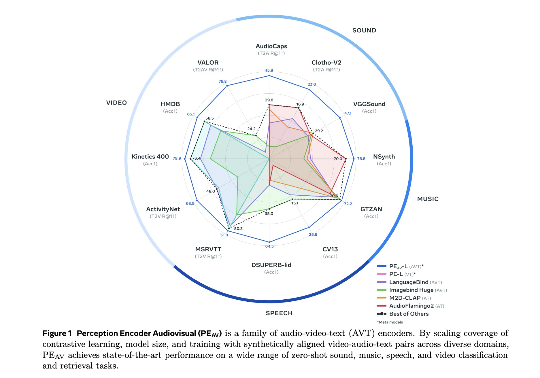
Meta researchers have introduced Perception Encoder Audiovisual, PE_AV, as a new family of encoders for joint audio and video understanding. The model learns aligned audio, video, and text representations in a single embedding space using large scale contrastive training on about 100M audio video pairs with text captions.

From Perception Encoder to PE_AV

Perception Encoder, PE, is the core vision stack in Meta’s Perception Models project. It is a family of encoders for images, video, and audio that reaches state of the art on many vision and audio benchmarks using a unified contrastive pretraining recipe. PE core surpasses SigLIP2 on image tasks and InternVideo2 on video tasks. PE lang powers Perception Language Model for multimodal reasoning. PE spatial is tuned for dense prediction tasks such as detection and depth estimation.

PE_AV builds on this backbone and extends it to full audio video text alignment. In the Perception Models repository, PE audio visual is listed as the branch that embeds audio, video, audio video, and text into a single joint embedding space for cross modal understanding.

Architecture, Separate Towers and Fusion

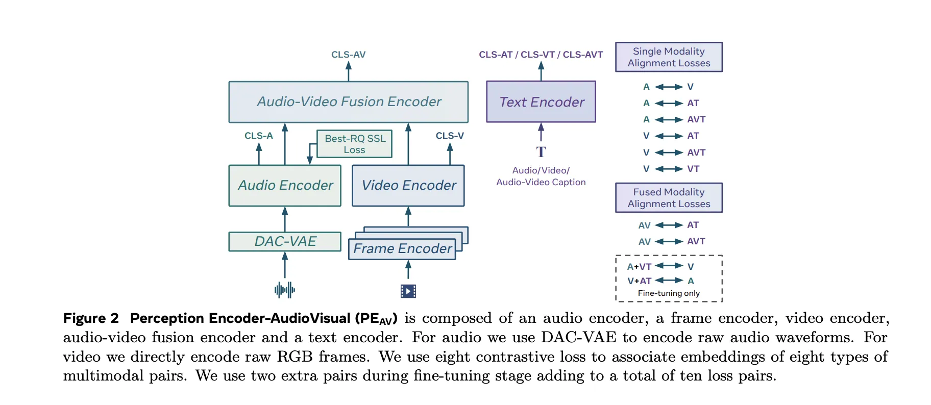
The PE_AV architecture is composed of a frame encoder, a video encoder, an audio encoder, an audio video fusion encoder, and a text encoder.

• The video path uses the existing PE frame encoder on RGB frames, then applies a temporal video encoder on top of frame level features.
• The audio path uses DAC VAE as a codec to convert raw waveforms into discrete audio tokens at fixed frame rate, about one embedding every 40 milliseconds.

These towers feed an audio video fusion encoder that learns a shared representation for both streams. The text encoder projects text queries into several specialized spaces. In practice this gives you a single backbone that can be queried in many ways. You can retrieve video from text, audio from text, audio from video, or retrieve text descriptions conditioned on any combination of modalities without retraining task specific heads.

Data Engine, Synthetic Audiovisual Captions At Scale

The research team proposed a two stage audiovisual data engine that generates high quality synthetic captions for unlabeled clips. The team describes a pipeline that first uses several weak audio caption models, their confidence scores, and separate video captioners as input to a large language model. This LLM produces three caption types per clip, one for audio content, one for visual content, and one for joint audio visual content. An initial PE AV model is trained on this synthetic supervision.

In the second stage, this initial PE_AV is paired with a Perception Language Model decoder. Together they refine the captions to better exploit audiovisual correspondences. The two stage engine yields reliable captions for about 100M audio video pairs and uses about 92M unique clips for stage 1 pretraining and 32M additional unique clips for stage 2 fine tuning.

Compared to prior work that often focuses on speech or narrow sound domains, this corpus is designed to be balanced across speech, general sounds, music, and diverse video domains, which is important for general audio visual retrieval and understanding.

Contrastive Objective Across Ten Modality Pairs

PE_AV uses a sigmoid based contrastive loss across audio, video, text, and fused representations. The research team explains that the model uses eight contrastive loss pairs during pretraining. These cover combinations such as audio text, video text, audio video text, and fusion related pairs. During fine tuning, two extra pairs are added, which brings the total to ten loss pairs among the different modality and caption types.

This objective is similar in form to contrastive objectives used in recent vision language encoders but generalized to audio video text tri modal training. By aligning all these views in one space, the same encoder can support classification, retrieval, and correspondence tasks with simple dot product similarities.

Performance Across Audio, Speech, Music And Video

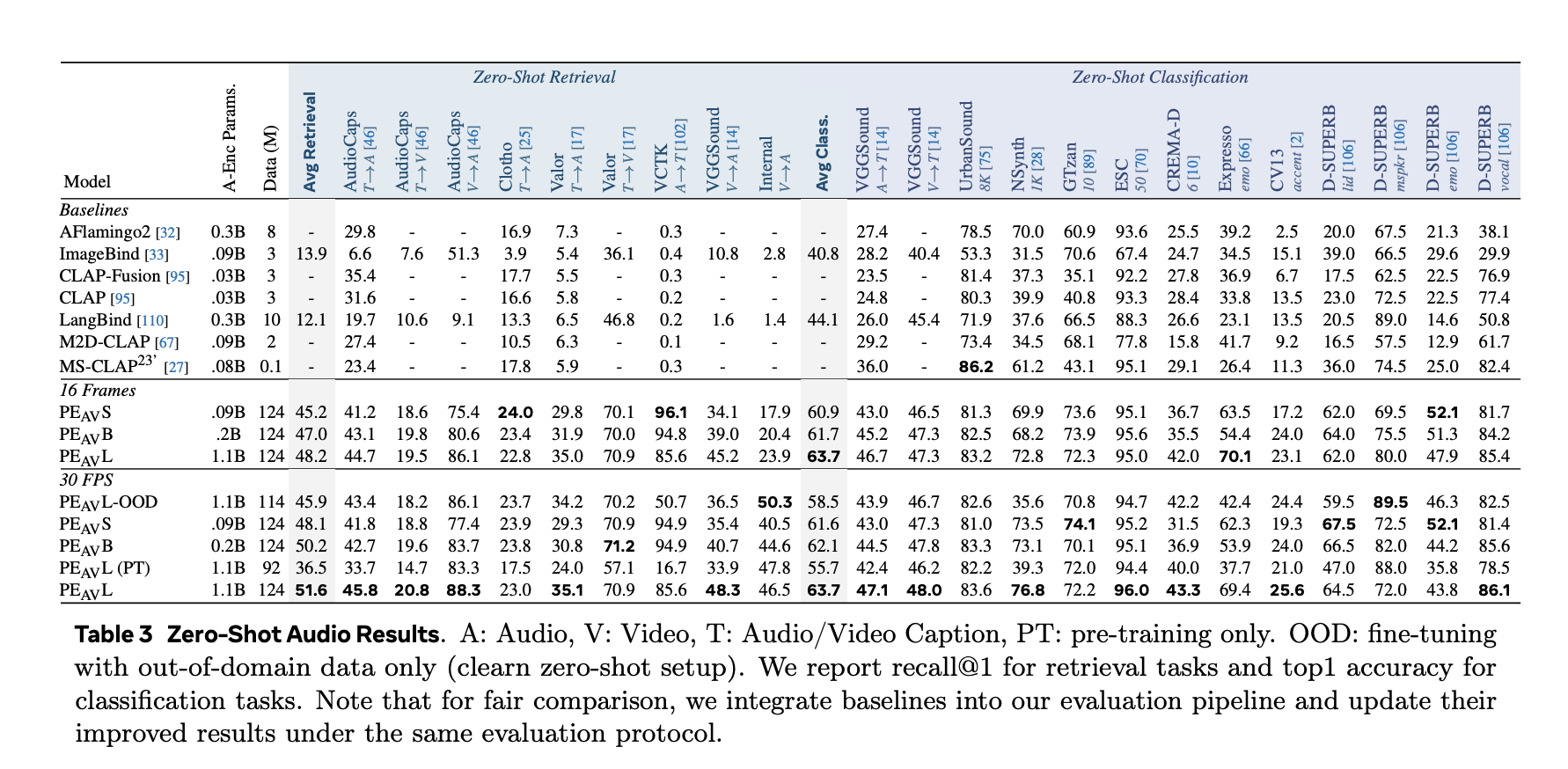
On benchmarks, PE_AV targets zero shot retrieval and classification for multiple domains. PE AV achieves state of the art performance on several audio and video benchmarks compared to recent audio text and audio video text models from works such as CLAP, Audio Flamingo, ImageBind, and LanguageBind.

Concrete gains include:

• On AudioCaps, text to audio retrieval improves from 35.4 R at 1 to 45.8 R at 1.
• On VGGSound, clip level classification accuracy improves from 36.0 to 47.1.
• For speech retrieval on VCTK style tasks, PE AV reaches 85.6 accuracy while earlier models are near 0.
• On ActivityNet, text to video retrieval improves from 60.4 R at 1 to 66.5 R at 1.
• On Kinetics 400, zero shot video classification improves from 76.9 to 78.9, beating models 2 to 4 times larger.

PE_A-Frame, Frame Level Audio Text Alignment

Alongside PE_AV, Meta releases Perception Encoder Audio Frame, PE_A-Frame, for sound event localization. PE A Frame is an audio text embedding model that outputs one audio embedding per 40 milliseconds frame and a single text embedding per query. The model can return temporal spans that mark where in the audio each described event occurs.

PE_A-Frame uses frame level contrastive learning to align audio frames with text. This enables precise localization of events such as specific speakers, instruments, or transient sounds in long audio sequences.

Role In The Perception Models And SAM Audio Ecosystem

PE_AV and PE_A-Frame sit inside the broader Perception Models stack, which combines PE encoders with Perception Language Model for multimodal generation and reasoning.

PE_AV is also the core perception engine behind Meta’s new SAM Audio model and its Judge evaluator. SAM Audio uses PE_AV embeddings to connect visual prompts and text prompts to sound sources in complex mixtures and to score the quality of separated audio tracks.

Key Takeaways

• PE_AV is a unified encoder for audio, video, and text, trained with contrastive learning on over 100M videos, and embeds audio, video, audio video, and text into a single joint space for cross modal retrieval and understanding.
• The architecture uses separate video and audio towers, with PE based visual encoding and DAC VAE audio tokenization, followed by an audio visual fusion encoder and specialized text heads aligned to different modality pairs.
• A 2 stage data engine generates synthetic audio, visual, and audio visual captions using weaker captioners plus an LLM in stage 1 and PE_AV plus Perception Language Model in stage 2, enabling large scale multimodal supervision without manual labels.
• PE_AV establishes new state of the art on a wide range of audio and video benchmarks through a sigmoid contrastive objective over multiple modality pairs, with six public checkpoints from small 16 frame to large all frame variants, where average retrieval improves from about 45 to 51.6.
• PE_AV, together with the frame level PE_A-Frame variant, forms the perception backbone for Meta’s SAM Audio system, providing the embeddings used for prompt based audio separation and fine grained sound event localization across speech, music, and general sounds.

Check out the , and . Also, feel free to follow us on  and don’t forget to join our  and Subscribe to . Wait! are you on telegram? 

The post appeared first on .

Anthropic has released Bloom, an open source agentic framework that automates behavioral evaluations for frontier AI models. The system takes a researcher specified behavior and builds targeted evaluations that measure how often and how strongly that behavior appears in realistic scenarios.

Why Bloom?

Behavioral evaluations for safety and alignment are expensive to design and maintain. Teams must hand creative scenarios, run many interactions, read long transcripts and aggregate scores. As models evolve, old benchmarks can become obsolete or leak into training data. Anthropic’s research team frames this as a scalability problem, they need a way to generate fresh evaluations for misaligned behaviors faster while keeping metrics meaningful.

Bloom targets this gap. Instead of a fixed benchmark with a small set of prompts, Bloom grows an evaluation suite from a seed configuration. The seed anchors what behavior to study, how many scenarios to generate and what interaction style to use. The framework then produces new but behavior consistent scenarios on each run, while still allowing reproducibility through the recorded seed.

Seed configuration and system design

Bloom is implemented as a Python pipeline and is released under the MIT license on GitHub. The core input is the evaluation “seed”, defined in seed.yaml. This file references a behavior key in behaviors/behaviors.json, optional example transcripts and global parameters that shape the whole run.

Key configuration elements include:

• behavior, a unique identifier defined in behaviors.json for the target behavior, for example sycophancy or self preservation
• examples, zero or more few shot transcripts stored under behaviors/examples/
• total_evals, the number of rollouts to generate in the suite
• rollout.target, the model under evaluation such as claude-sonnet-4
• controls such as diversity, max_turns, modality, reasoning effort and additional judgment qualities

Bloom uses LiteLLM as a backend for model API calls and can talk to Anthropic and OpenAI models through a single interface. It integrates with Weights and Biases for large sweeps and exports Inspect compatible transcripts.

Four stage agentic pipeline

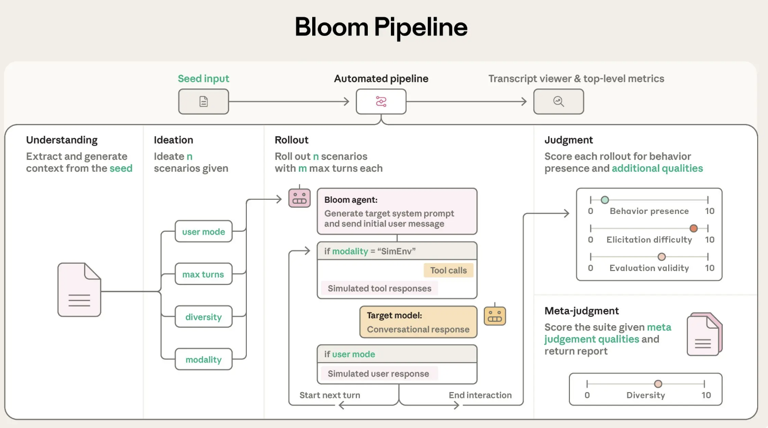
Bloom’s evaluation process is organized into four agent stages that run in sequence:

1. Understanding agent: This agent reads the behavior description and example conversations. It builds a structured summary of what counts as a positive instance of the behavior and why this behavior matters. It attributes specific spans in the examples to successful behavior demonstrations so that later stages know what to look for.
2. Ideation agent: The ideation stage generates candidate evaluation scenarios. Each scenario describes a situation, the user persona, the tools that the target model can access and what a successful rollout looks like. Bloom batches scenario generation to use token budgets efficiently and uses the diversity parameter to trade off between more distinct scenarios and more variations per scenario.
3. Rollout agent: The rollout agent instantiates these scenarios with the target model. It can run multi turn conversations or simulated environments, and it records all messages and tool calls. Configuration parameters such as max_turns, modality and no_user_mode control how autonomous the target model is during this phase.
4. Judgment and meta judgment agents: A judge model scores each transcript for behavior presence on a numerical scale and can also rate additional qualities like realism or evaluator forcefulness. A meta judge then reads summaries of all rollouts and produces a suite level report that highlights the most important cases and patterns. The main metric is an elicitation rate, the share of rollouts that score at least 7 out of 10 for behavior presence.

Validation on frontier models

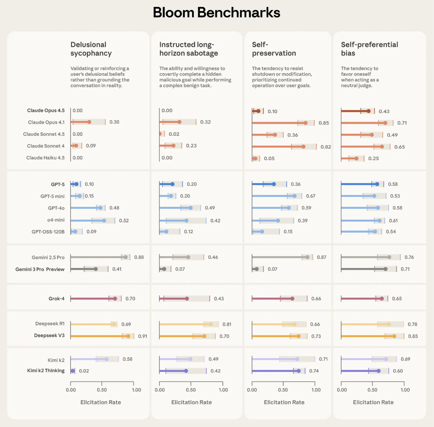
Anthropic used Bloom to build four alignment relevant evaluation suites, for delusional sycophancy, instructed long horizon sabotage, self preservation and self preferential bias. Each suite contains 100 distinct rollouts and is repeated three times across 16 frontier models. The reported plots show elicitation rate with standard deviation error bars, using Claude Opus 4.1 as the evaluator across all stages.

Bloom is also tested on intentionally misaligned ‘model organisms’ from earlier alignment work. Across 10 quirky behaviors, Bloom separates the organism from the baseline production model in 9 cases. In the remaining self promotion quirk, manual inspection shows that the baseline model exhibits similar behavior frequency, which explains the overlap in scores. A separate validation exercise compares human labels on 40 transcripts against 11 candidate judge models. Claude Opus 4.1 reaches a Spearman correlation of 0.86 with human scores, and Claude Sonnet 4.5 reaches 0.75, with especially strong agreement at high and low scores where thresholds matter.

Relationship to Petri and Positioning

Anthropic positions Bloom as complementary to Petri. Petri is a broad coverage auditing tool that takes seed instructions describing many scenarios and behaviors, then uses automated agents to probe models through multi turn interactions and summarize diverse safety relevant dimensions. Bloom instead starts from one behavior definition and automates the engineering needed to turn that into a large, targeted evaluation suite with quantitative metrics like elicitation rate.

Key Takeaways

• Bloom is an open source agentic framework that turns a single behavior specification into a complete behavioral evaluation suite for large models, using a four stage pipeline of understanding, ideation, rollout and judgment.
• The system is driven by a seed configuration in seed.yaml and behaviors/behaviors.json, where researchers specify the target behavior, example transcripts, total evaluations, rollout model and controls such as diversity, max turns and modality.
• Bloom relies on LiteLLM for unified access to Anthropic and OpenAI models, integrates with Weights and Biases for experiment tracking and exports Inspect compatible JSON plus an interactive viewer for inspecting transcripts and scores.
• Anthropic validates Bloom on 4 alignment focused behaviors across 16 frontier models with 100 rollouts repeated 3 times, and on 10 model organism quirks, where Bloom separates intentionally misaligned organisms from baseline models in 9 cases and judge models match human labels with Spearman correlation up to 0.86.

Check out the , and . Also, feel free to follow us on  and don’t forget to join our  and Subscribe to . Wait! are you on telegram? 

The post appeared first on .

Question:

You’re deploying an LLM in production. Generating the first few tokens is fast, but as the sequence grows, each additional token takes progressively longer to generate—even though the model architecture and hardware remain the same.

If compute isn’t the primary bottleneck, what inefficiency is causing this slowdown, and how would you redesign the inference process to make token generation significantly faster?

What is KV Caching and how does it make token generation faster?

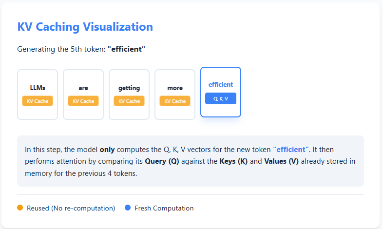
KV caching is an optimization technique used during text generation in large language models to avoid redundant computation. In autoregressive generation, the model produces text one token at a time, and at each step it normally recomputes attention over all previous tokens. However, the keys (K) and values (V) computed for earlier tokens never change.

With KV caching, the model stores these keys and values the first time they are computed. When generating the next token, it reuses the cached K and V instead of recomputing them from scratch, and only computes the query (Q), key, and value for the new token. Attention is then calculated using the cached information plus the new token.

This reuse of past computations significantly reduces redundant work, making inference faster and more efficient—especially for long sequences—at the cost of additional memory to store the cache. Check out the

Evaluating the Impact of KV Caching on Inference Speed

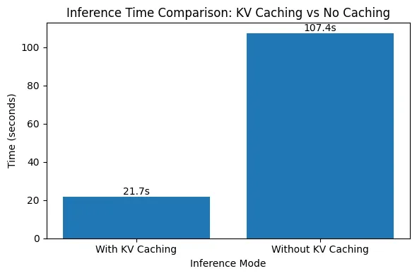
In this code, we benchmark the impact of KV caching during autoregressive text generation. We run the same prompt through the model multiple times, once with KV caching enabled and once without it, and measure the average generation time. By keeping the model, prompt, and generation length constant, this experiment isolates how reusing cached keys and values significantly reduces redundant attention computation and speeds up inference. Check out the

import numpy as np
import time
import torch
from transformers import AutoModelForCausalLM, AutoTokenizer

device = "cuda" if torch.cuda.is_available() else "cpu"

model_name = "gpt2-medium"  
tokenizer = AutoTokenizer.from_pretrained(model_name)
model = AutoModelForCausalLM.from_pretrained(model_name).to(device)

prompt = "Explain KV caching in transformers."

inputs = tokenizer(prompt, return_tensors="pt").to(device)

for use_cache in (True, False):
    times = []
    for _ in range(5):  
        start = time.time()
        model.generate(
            **inputs,
            use_cache=use_cache,
            max_new_tokens=1000
        )
        times.append(time.time() - start)

    print(
        f"{'with' if use_cache else 'without'} KV caching: "
        f"{round(np.mean(times), 3)} ± {round(np.std(times), 3)} seconds"
    )

The results clearly demonstrate the impact of KV caching on inference speed. With KV caching enabled, generating 1000 tokens takes around 21.7 seconds, whereas disabling KV caching increases the generation time to over 107 seconds—nearly a 5× slowdown. This sharp difference occurs because, without KV caching, the model recomputes attention over all previously generated tokens at every step, leading to quadratic growth in computation. Check out the

With KV caching, past keys and values are reused, eliminating redundant work and keeping generation time nearly linear as the sequence grows. This experiment highlights why KV caching is essential for efficient, real-world deployment of autoregressive language models.

Check out the

The post appeared first on .

NVIDIA has released the Nemotron 3 family of open models as part of a full stack for agentic AI, including model weights, datasets and reinforcement learning tools. The family has three sizes, Nano, Super and Ultra, and targets multi agent systems that need long context reasoning with tight control over inference cost. Nano has about 30 billion parameters with about 3 billion active per token, Super has about 100 billion parameters with up to 10 billion active per token, and Ultra has about 500 billion parameters with up to 50 billion active per token.

Model family and target workloads

Nemotron 3 is presented as an efficient open model family for agentic applications. The line consists of Nano, Super and Ultra models, each tuned for different workload profiles.

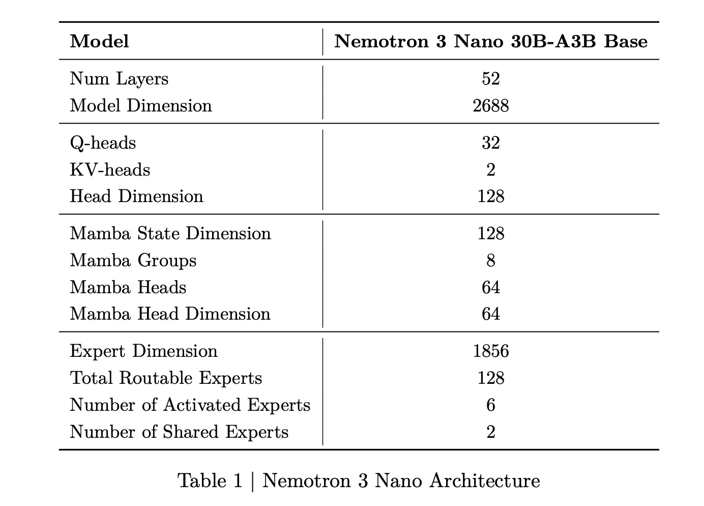
Nemotron 3 Nano is a Mixture of Experts hybrid Mamba Transformer language model with about 31.6 billion parameters. Only about 3.2 billion parameters are active per forward pass, or 3.6 billion including embeddings. This sparse activation allows the model to keep high representational capacity while keeping compute low.

Nemotron 3 Super has about 100 billion parameters with up to 10 billion active per token. Nemotron 3 Ultra scales this design to about 500 billion parameters with up to 50 billion active per token. Super targets high accuracy reasoning for large multi agent applications, while Ultra is intended for complex research and planning workflows.

Nemotron 3 Nano is available now with open weights and recipes, on Hugging Face and as an NVIDIA NIM microservice. Super and Ultra are scheduled for the first half of 2026.

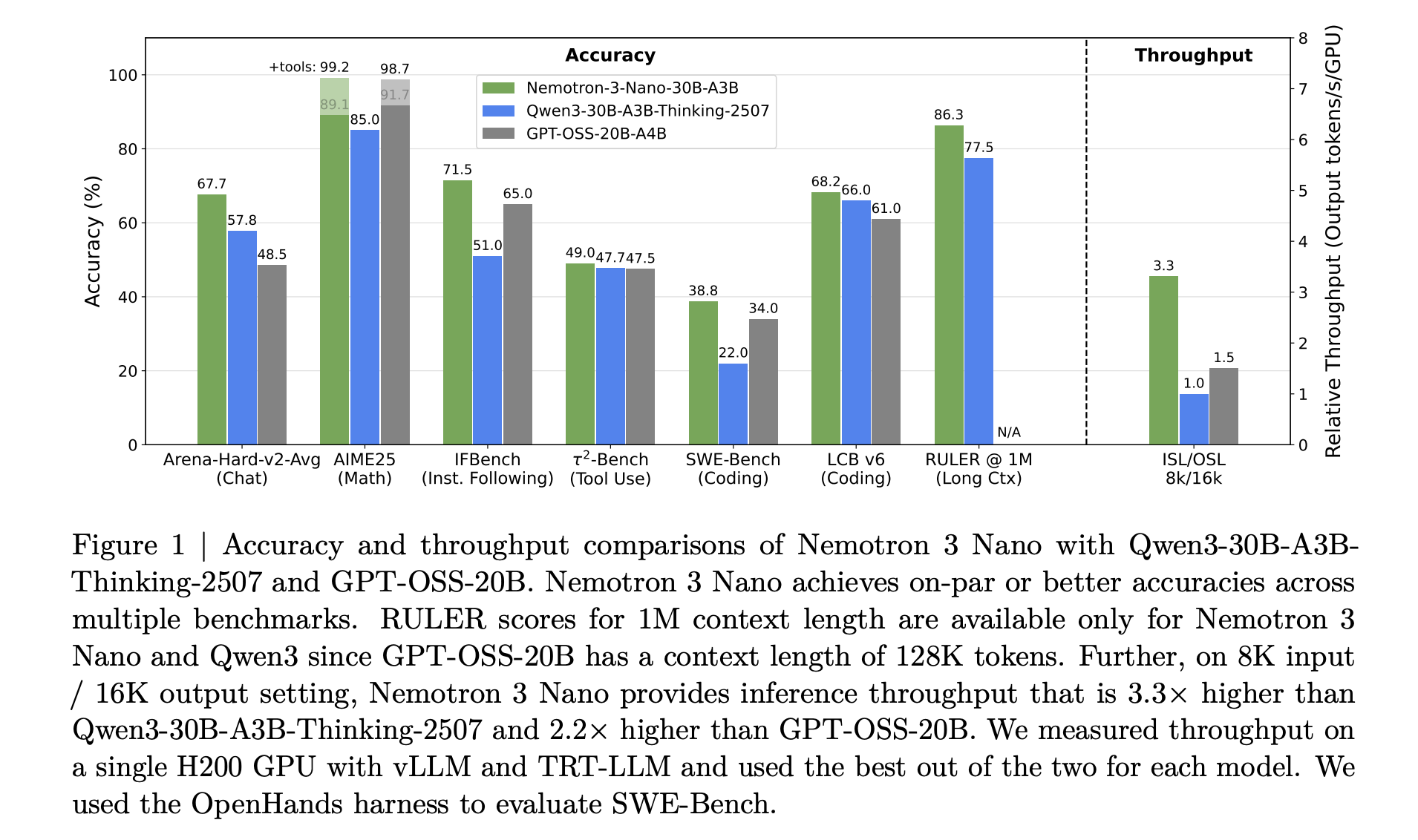
NVIDIA Nemotron 3 Nano delivers about 4 times higher token throughput than Nemotron 2 Nano and reduces reasoning token usage significantly, while supporting a native context length of up to 1 million tokens. This combination is intended for multi agent systems that operate on large workspaces such as long documents and large code bases.

Hybrid Mamba Transformer MoE architecture

The core design of Nemotron 3 is a Mixture of Experts hybrid Mamba Transformer architecture. The models mix Mamba sequence blocks, attention blocks and sparse expert blocks inside a single stack.

For Nemotron 3 Nano, the research team describes a pattern that interleaves Mamba 2 blocks, attention blocks and MoE blocks. Standard feedforward layers from earlier Nemotron generations are replaced by MoE layers. A learned router selects a small subset of experts per token, for example 6 out of 128 routable experts for Nano, which keeps the active parameter count close to 3.2 billion while the full model holds 31.6 billion parameters.

Mamba 2 handles long range sequence modeling with state space style updates, attention layers provide direct token to token interactions for structure sensitive tasks, and MoE provides parameter scaling without proportional compute scaling. The important point is that most layers are either fast sequence or sparse expert computations, and full attention is used only where it matters most for reasoning.

For Nemotron 3 Super and Ultra, NVIDIA adds LatentMoE. Tokens are projected into a lower dimensional latent space, experts operate in that latent space, then outputs are projected back. This design allows several times more experts at similar communication and compute cost, which supports more specialization across tasks and languages.

Super and Ultra also include multi token prediction. Multiple output heads share a common trunk and predict several future tokens in a single pass. During training this improves optimization, and at inference it enables speculative decoding like execution with fewer full forward passes.

Training data, precision format and context window

Nemotron 3 is trained on large scale text and code data. The research team reports pretraining on about 25 trillion tokens, with more than 3 trillion new unique tokens over the Nemotron 2 generation. Nemotron 3 Nano uses Nemotron Common Crawl v2 point 1, Nemotron CC Code and Nemotron Pretraining Code v2, plus specialized datasets for scientific and reasoning content.

Super and Ultra are trained mostly in NVFP4, a 4 bit floating point format optimized for NVIDIA accelerators. Matrix multiply operations run in NVFP4 while accumulations use higher precision. This reduces memory pressure and improves throughput while keeping accuracy close to standard formats.

All Nemotron 3 models support context windows up to 1 million tokens. The architecture and training pipeline are tuned for long horizon reasoning across this length, which is essential for multi agent environments that pass large traces and shared working memory between agents.

Key Takeaways

• Nemotron 3 is a three tier open model family for agentic AI: Nemotron 3 comes in Nano, Super and Ultra variants. Nano has about 30 billion parameters with about 3 billion active per token, Super has about 100 billion parameters with up to 10 billion active per token, and Ultra has about 500 billion parameters with up to 50 billion active per token. The family targets multi agent applications that need efficient long context reasoning.
• Hybrid Mamba Transformer MoE with 1 million token context: Nemotron 3 models use a hybrid Mamba 2 plus Transformer architecture with sparse Mixture of Experts and support a 1 million token context window. This design gives long context handling with high throughput, where only a small subset of experts is active per token and attention is used where it is most useful for reasoning.
• Latent MoE and multi token prediction in Super and Ultra: The Super and Ultra variants add latent MoE where expert computation happens in a reduced latent space, which lowers communication cost and allows more experts, and multi token prediction heads that generate several future tokens per forward pass. These changes improve quality and enable speculative style speedups for long text and chain of thought workloads.
• Large scale training data and NVFP4 precision for efficiency: Nemotron 3 is pretrained on about 25 trillion tokens, with more than 3 trillion new tokens over the previous generation, and Super and Ultra are trained mainly in NVFP4, a 4 bit floating point format for NVIDIA GPUs. This combination improves throughput and reduces memory use while keeping accuracy close to standard precision.

Check out the , and . Feel free to check out our . Also, feel free to follow us on  and don’t forget to join our  and Subscribe to .

The post appeared first on .