Tencent Hunyuan’s 3D Digital Human team has released HY-Motion 1.0, an open weight text-to-3D human motion generation family that scales Diffusion Transformer based Flow Matching to 1B parameters in the motion domain. The models turn natural language prompts plus an expected duration into 3D human motion clips on a unified SMPL-H skeleton and are available on GitHub and Hugging Face with code, checkpoints and a Gradio interface for local use.

What HY-Motion 1.0 provides for developers?

HY-Motion 1.0 is a series of text-to-3D human motion generation models built on a Diffusion Transformer, DiT, trained with a Flow Matching objective. The model series showcases 2 variants, HY-Motion-1.0 with 1.0B parameters as the standard model and HY-Motion-1.0-Lite with 0.46B parameters as a lightweight option.

Both models generate skeleton based 3D character animations from simple text prompts. The output is a motion sequence on an SMPL-H skeleton that can be integrated into 3D animation or game pipelines, for example for digital humans, cinematics and interactive characters. The release includes inference scripts, a batch oriented CLI and a Gradio web app, and supports macOS, Windows and Linux.

Data engine and taxonomy

The training data comes from 3 sources, in the wild human motion videos, motion capture data and 3D animation assets for game production. The research team starts from 12M high quality video clips from HunyuanVideo, runs shot boundary detection to split scenes and a human detector to keep clips with people, then applies the GVHMR algorithm to reconstruct SMPL X motion tracks. Motion capture sessions and 3D animation libraries contribute about 500 hours of additional motion sequences.

All data is retargeted onto a unified SMPL-H skeleton through mesh fitting and retargeting tools. A multi stage filter removes duplicate clips, abnormal poses, outliers in joint velocity, anomalous displacements, long static segments and artifacts such as foot sliding. Motions are then canonicalized, resampled to 30 fps and segmented into clips shorter than 12 seconds with a fixed world frame, Y axis up and the character facing the positive Z axis. The final corpus contains over 3,000 hours of motion, of which 400 hours are high quality 3D motion with verified captions.

On top of this, the research team defines a 3 level taxonomy. At the top level there are 6 classes, Locomotion, Sports and Athletics, Fitness and Outdoor Activities, Daily Activities, Social Interactions and Leisure and Game Character Actions. These expand into more than 200 fine grained motion categories at the leaves, which cover both simple atomic actions and concurrent or sequential motion combinations.

Motion representation and HY-Motion DiT

HY-Motion 1.0 uses the SMPL-H skeleton with 22 body joints without hands. Each frame is a 201 dimensional vector that concatenates global root translation in 3D space, global body orientation in a continuous 6D rotation representation, 21 local joint rotations in 6D form and 22 local joint positions in 3D coordinates. Velocities and foot contact labels are removed because they slowed training and did not help final quality. This representation is compatible with animation workflows and close to the DART model representation.

The core network is a hybrid HY Motion DiT. It first applies dual stream blocks that process motion latents and text tokens separately. In these blocks, each modality has its own QKV projections and MLP, and a joint attention module allows motion tokens to query semantic features from text tokens while keeping modality specific structure. The network then switches to single stream blocks that concatenate motion and text tokens into one sequence and process them with parallel spatial and channel attention modules to perform deeper multimodal fusion.

For text conditioning, the system uses a dual encoder scheme. Qwen3 8B provides token level embeddings, while a CLIP-L model provides global text features. A Bidirectional Token Refiner fixes the causal attention bias of the LLM for non autoregressive generation. These signals feed the DiT through adaptive layer normalization conditioning. Attention is asymmetric, motion tokens can attend to all text tokens, but text tokens do not attend back to motion, which prevents noisy motion states from corrupting the language representation. Temporal attention inside the motion branch uses a narrow sliding window of 121 frames, which focuses capacity on local kinematics while keeping cost manageable for long clips. Full Rotary Position Embedding is applied after concatenating text and motion tokens to encode relative positions across the whole sequence.

Flow Matching, prompt rewriting and training

HY-Motion 1.0 uses Flow Matching instead of standard denoising diffusion. The model learns a velocity field along a continuous path that interpolates between Gaussian noise and real motion data. During training, the objective is a mean squared error between predicted and ground truth velocities along this path. During inference, the learned ordinary differential equation is integrated from noise to a clean trajectory, which gives stable training for long sequences and fits the DiT architecture.

A separate Duration Prediction and Prompt Rewrite module improves instruction following. It uses Qwen3 30B A3B as the base model and is trained on synthetic user style prompts generated from motion captions with a VLM and LLM pipeline, for example Gemini 2.5 Pro. This module predicts a suitable motion duration and rewrites informal prompts into normalized text that is easier for the DiT to follow. It is trained first with supervised fine tuning and then refined with Group Relative Policy Optimization, using Qwen3 235B A22B as a reward model that scores semantic consistency and duration plausibility.

Training follows a 3 stage curriculum. Stage 1 performs large scale pretraining on the full 3,000 hour dataset to learn a broad motion prior and basic text motion alignment. Stage 2 fine tunes on the 400 hour high quality set to sharpen motion detail and improve semantic correctness with a smaller learning rate. Stage 3 applies reinforcement learning, first Direct Preference Optimization using 9,228 curated human preference pairs sampled from about 40,000 generated pairs, then Flow GRPO with a composite reward. The reward combines a semantic score from a Text Motion Retrieval model and a physics score that penalizes artifacts like foot sliding and root drift, under a KL regularization term to stay close to the supervised model.

Benchmarks, scaling behavior and limitations

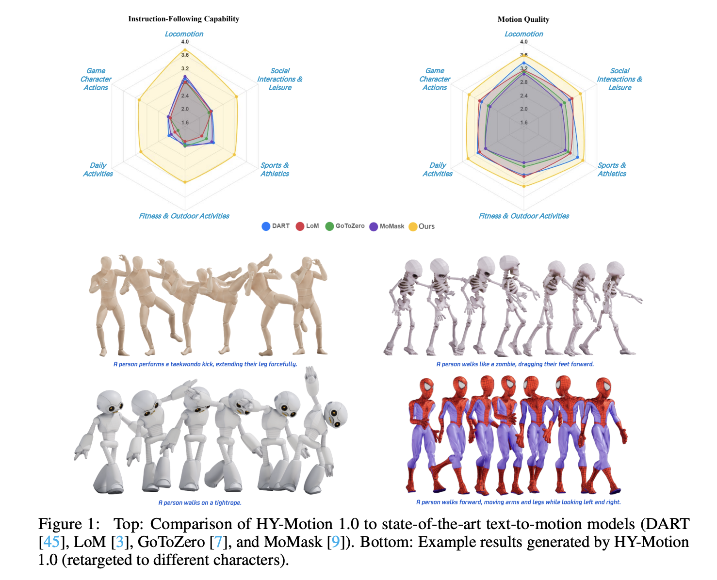
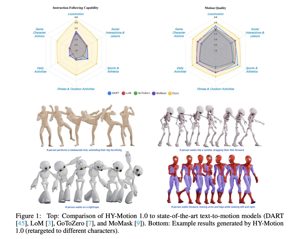
For evaluation, the team builds a test set of over 2,000 prompts that span the 6 taxonomy categories and include simple, concurrent and sequential actions. Human raters score instruction following and motion quality on a scale from 1 to 5. HY-Motion 1.0 reaches an average instruction following score of 3.24 and an SSAE score of 78.6 percent. Baseline text-to-motion systems such as DART, LoM, GoToZero and MoMask achieve scores between 2.17 and 2.31 with SSAE between 42.7 percent and 58.0 percent. For motion quality, HY-Motion 1.0 reaches 3.43 on average versus 3.11 for the best baseline.

Scaling experiments study DiT models with 0.05B, 0.46B, 0.46B trained only on 400 hours and 1B parameters. Instruction following improves steadily with model size, with the 1B model reaching an average of 3.34. Motion quality saturates around the 0.46B scale, where the 0.46B and 1B models reach similar averages between 3.26 and 3.34. Comparison of the 0.46B model trained on 3,000 hours and the 0.46B model trained only on 400 hours shows that larger data volume is key for instruction alignment, while high quality curation mainly improves realism.

Key Takeaways

• Billion scale DiT Flow Matching for motion: HY-Motion 1.0 is the first Diffusion Transformer based Flow Matching model scaled to the 1B parameter level specifically for text to 3D human motion, targeting high fidelity instruction following across diverse actions.
• Large scale, curated motion corpus: The model is pretrained on over 3,000 hours of reconstructed, mocap and animation motion data and fine tuned on a 400 hour high quality subset, all retargeted to a unified SMPL H skeleton and organized into more than 200 motion categories.
• Hybrid DiT architecture with strong text conditioning: HY-Motion 1.0 uses a hybrid dual stream and single stream DiT with asymmetric attention, narrow band temporal attention and dual text encoders, Qwen3 8B and CLIP L, to fuse token level and global semantics into motion trajectories.
• RL aligned prompt rewrite and training pipeline: A dedicated Qwen3 30B based module predicts motion duration and rewrites user prompts, and the DiT is further aligned with Direct Preference Optimization and Flow GRPO using semantic and physics rewards, which improves realism and instruction following beyond supervised training.

Check out the  and  Also, feel free to follow us on  and don’t forget to join our  and Subscribe to . Wait! are you on telegram? 

The post appeared first on .

LLMRouter is an open source routing library from the U Lab at the University of Illinois Urbana Champaign that treats model selection as a first class system problem. It sits between applications and a pool of LLMs and chooses a model for each query based on task complexity, quality targets, and cost, all exposed through a unified Python API and CLI. The project ships with more than 16 routing models, a data generation pipeline over 11 benchmarks, and a plugin system for custom routers.

Router families and supported models

LLMRouter organizes routing algorithms into four families, Single-Round Routers, Multi-Round Routers, Personalized Routers, and Agentic Routers. Single round routers include knnrouter, svmrouter, mlprouter, mfrouter, elorouter, routerdc, automix, hybrid_llm, graphrouter, causallm_router, and the baselines smallest_llm and largest_llm. These models implement strategies such as k nearest neighbors, support vector machines, multilayer perceptrons, matrix factorization, Elo rating, dual contrastive learning, automatic model mixing, and graph based routing.

Multi round routing is exposed through router_r1, a pre trained instance of Router R1 integrated into LLMRouter. Router R1 formulates multi LLM routing and aggregation as a sequential decision process where the router itself is an LLM that alternates between internal reasoning steps and external model calls. It is trained with reinforcement learning using a rule based reward that balances format, outcome, and cost. In LLMRouter, router_r1 is available as an extra installation target with pinned dependencies tested on vllm==0.6.3 and torch==2.4.0.

Personalized routing is handled by gmtrouter, described as a graph based personalized router with user preference learning. GMTRouter represents multi turn user LLM interactions as a heterogeneous graph over users, queries, responses, and models. It runs a message passing architecture over this graph to infer user specific routing preferences from few shot interaction data, and experiments show accuracy and AUC gains over non personalized baselines.

Agentic routers in LLMRouter extend routing to multi step reasoning workflows. knnmultiroundrouter uses k nearest neighbor reasoning over multi turn traces and is intended for complex tasks. llmmultiroundrouter exposes an LLM based agentic router that performs multi step routing without its own training loop. These agentic routers share the same configuration and data formats as the other router families and can be swapped through a single CLI flag.

Data generation pipeline for routing datasets

LLMRouter ships with a full data generation pipeline that turns standard benchmarks and LLM outputs into routing datasets. The pipeline supports 11 benchmarks, Natural QA, Trivia QA, MMLU, GPQA, MBPP, HumanEval, GSM8K, CommonsenseQA, MATH, OpenBookQA, and ARC Challenge. It runs in three explicit stages. First, data_generation.py extracts queries and ground truth labels and creates train and test JSONL splits. Second, generate_llm_embeddings.py builds embeddings for candidate LLMs from metadata. Third, api_calling_evaluation.py calls LLM APIs, evaluates responses, and fuses scores with embeddings into routing records. ()

The pipeline outputs query files, LLM embedding JSON, query embedding tensors, and routing data JSONL files. A routing entry includes fields such as task_name, query, ground_truth, metric, model_name, response, performance, embedding_id, and token_num. Configuration is handled entirely through YAML, so engineers point the scripts to new datasets and candidate model lists without modifying code.

Chat interface and plugin system

For interactive use, llmrouter chat launches a Gradio based chat frontend over any router and configuration. The server can bind to a custom host and port and can expose a public sharing link. Query modes control how routing sees context. current_only uses only the latest user message, full_context concatenates the dialogue history, and retrieval augments the query with the top k similar historical queries. The UI visualizes model choices in real time and is driven by the same router configuration used for batch inference.

LLMRouter also provides a plugin system for custom routers. New routers live under custom_routers, subclass MetaRouter, and implement route_single and route_batch. Configuration files under that directory define data paths, hyperparameters, and optional default API endpoints. Plugin discovery scans the project custom_routers folder, a ~/.llmrouter/plugins directory, and any extra paths in the LLMROUTER_PLUGINS environment variable. Example custom routers include randomrouter, which selects a model at random, and thresholdrouter, which is a trainable router that estimates query difficulty.

Key Takeaways

• Routing as a first class abstraction: LLMRouter is an open source routing layer from UIUC that sits between applications and heterogeneous LLM pools and centralizes model selection as a cost and quality aware prediction task rather than ad hoc scripts.
• Four router families covering 16 plus algorithms: The library standardizes more than 16 routers into four families, single round, multi round, personalized, and agentic, including knnrouter, graphrouter, routerdc, router_r1, and gmtrouter, all exposed through a unified config and CLI.
• Multi round RL routing via Router R1: router_r1 integrates the Router R1 framework, where an LLM router interleaves internal “think” steps with external “route” calls and is trained with a rule based reward that combines format, outcome, and cost to optimize performance cost trade offs.
• Graph based personalization with GMTRouter: gmtrouter models users, queries, responses and LLMs as nodes in a heterogeneous graph and uses message passing to learn user specific routing preferences from few shot histories, achieving up to around 21% accuracy gains and substantial AUC improvements over strong baselines.
• End to end pipeline and extensibility: LLMRouter provides a benchmark driven data pipeline, CLI for training and inference, a Gradio chat UI, centralized API key handling, and a plugin system based on MetaRouter that allows teams to register custom routers while reusing the same routing datasets and infrastructure.

Check out the  and . Also, feel free to follow us on  and don’t forget to join our  and Subscribe to . Wait! are you on telegram? 

The post appeared first on .

In this tutorial, we build an advanced, end-to-end multi-agent research workflow using the framework. We design a coordinated society of agents, Planner, Researcher, Writer, Critic, and Finalizer, that collaboratively transform a high-level topic into a polished, evidence-grounded research brief. We securely integrate the OpenAI API, orchestrate agent interactions programmatically, and add lightweight persistent memory to retain knowledge across runs. By structuring the system around clear roles, JSON-based contracts, and iterative refinement, we demonstrate how CAMEL can be used to construct reliable, controllable, and scalable agentic pipelines. Check out the .

!pip -q install "camel-ai[all]" "python-dotenv" "rich"


import os
import json
import time
from typing import Dict, Any
from rich import print as rprint


def load_openai_key() -> str:
   key = None
   try:
       from google.colab import userdata
       key = userdata.get("OPENAI_API_KEY")
   except Exception:
       key = None
   if not key:
       import getpass
       key = getpass.getpass("Enter OPENAI_API_KEY (hidden): ").strip()
   if not key:
       raise ValueError("OPENAI_API_KEY is required.")
   return key


os.environ["OPENAI_API_KEY"] = load_openai_key()

We set up the execution environment and securely load the OpenAI API key using Colab secrets or a hidden prompt. We ensure the runtime is ready by installing dependencies and configuring authentication so the workflow can run safely without exposing credentials. Check out the .

from camel.models import ModelFactory
from camel.types import ModelPlatformType, ModelType
from camel.agents import ChatAgent
from camel.toolkits import SearchToolkit


MODEL_CFG = {"temperature": 0.2}


model = ModelFactory.create(
   model_platform=ModelPlatformType.OPENAI,
   model_type=ModelType.GPT_4O,
   model_config_dict=MODEL_CFG,
)

We initialize the CAMEL model configuration and create a shared language model instance using the ModelFactory abstraction. We standardize model behavior across all agents to ensure consistent, reproducible reasoning throughout the multi-agent pipeline. Check out the .

MEM_PATH = "camel_memory.json"


def mem_load() -> Dict[str, Any]:
   if not os.path.exists(MEM_PATH):
       return {"runs": []}
   with open(MEM_PATH, "r", encoding="utf-8") as f:
       return json.load(f)


def mem_save(mem: Dict[str, Any]) -> None:
   with open(MEM_PATH, "w", encoding="utf-8") as f:
       json.dump(mem, f, ensure_ascii=False, indent=2)


def mem_add_run(topic: str, artifacts: Dict[str, str]) -> None:
   mem = mem_load()
   mem["runs"].append({"ts": int(time.time()), "topic": topic, "artifacts": artifacts})
   mem_save(mem)


def mem_last_summaries(n: int = 3) -> str:
   mem = mem_load()
   runs = mem.get("runs", [])[-n:]
   if not runs:
       return "No past runs."
   return "n".join([f"{i+1}. topic={r['topic']} | ts={r['ts']}" for i, r in enumerate(runs)])

We implement a lightweight persistent memory layer backed by a JSON file. We store artifacts from each run and retrieve summaries of previous executions, allowing us to introduce continuity and historical context across sessions. Check out the .

def make_agent(role: str, goal: str, extra_rules: str = "") -> ChatAgent:
   system = (
       f"You are {role}.n"
       f"Goal: {goal}n"
       f"{extra_rules}n"
       "Output must be crisp, structured, and directly usable by the next agent."
   )
   return ChatAgent(model=model, system_message=system)


planner = make_agent(
   "Planner",
   "Create a compact plan and research questions with acceptance criteria.",
   "Return JSON with keys: plan, questions, acceptance_criteria."
)


researcher = make_agent(
   "Researcher",
   "Answer questions using web search results.",
   "Return JSON with keys: findings, sources, open_questions."
)


writer = make_agent(
   "Writer",
   "Draft a structured research brief.",
   "Return Markdown only."
)


critic = make_agent(
   "Critic",
   "Identify weaknesses and suggest fixes.",
   "Return JSON with keys: issues, fixes, rewrite_instructions."
)


finalizer = make_agent(
   "Finalizer",
   "Produce the final improved brief.",
   "Return Markdown only."
)


search_tool = SearchToolkit().search_duckduckgo
researcher = ChatAgent(
   model=model,
   system_message=researcher.system_message,
   tools=[search_tool],
)

We define the core agent roles and their responsibilities within the workflow. We construct specialized agents with clear goals and output contracts, and we enhance the Researcher by attaching a web search tool for evidence-grounded responses. Check out the .

def step_json(agent: ChatAgent, prompt: str) -> Dict[str, Any]:
   res = agent.step(prompt)
   txt = res.msgs[0].content.strip()
   try:
       return json.loads(txt)
   except Exception:
       return {"raw": txt}


def step_text(agent: ChatAgent, prompt: str) -> str:
   res = agent.step(prompt)
   return res.msgs[0].content

We abstract interaction patterns with agents into helper functions that enforce structured JSON or free-text outputs. We simplify orchestration by handling parsing and fallback logic centrally, making the pipeline more robust to formatting variability. Check out the .

def run_workflow(topic: str) -> Dict[str, str]:
   rprint(mem_last_summaries(3))


   plan = step_json(
       planner,
       f"Topic: {topic}nCreate a tight plan and research questions."
   )


   research = step_json(
       researcher,
       f"Research the topic using web search.n{json.dumps(plan)}"
   )


   draft = step_text(
       writer,
       f"Write a research brief using:n{json.dumps(research)}"
   )


   critique = step_json(
       critic,
       f"Critique the draft:n{draft}"
   )


   final = step_text(
       finalizer,
       f"Rewrite using critique:n{json.dumps(critique)}nDraft:n{draft}"
   )


   artifacts = {
       "plan_json": json.dumps(plan, indent=2),
       "research_json": json.dumps(research, indent=2),
       "draft_md": draft,
       "critique_json": json.dumps(critique, indent=2),
       "final_md": final,
   }


   mem_add_run(topic, artifacts)
   return artifacts


TOPIC = "Agentic multi-agent research workflow with quality control"
artifacts = run_workflow(TOPIC)
print(artifacts["final_md"])

We orchestrate the complete multi-agent workflow from planning to finalization. We sequentially pass artifacts between agents, apply critique-driven refinement, persist results to memory, and produce a finalized research brief ready for downstream use.

In conclusion, we implemented a practical CAMEL-based multi-agent system that mirrors real-world research and review workflows. We showed how clearly defined agent roles, tool-augmented reasoning, and critique-driven refinement lead to higher-quality outputs while reducing hallucinations and structural weaknesses. We also established a foundation for extensibility by persisting artifacts and enabling reuse across sessions. This approach allows us to move beyond single-prompt interactions and toward robust agentic systems that can be adapted for research, analysis, reporting, and decision-support tasks at scale.

Check out the . Also, feel free to follow us on  and don’t forget to join our  and Subscribe to . Wait! are you on telegram? 

The post appeared first on .

In this tutorial, we demonstrate how to design a contract-first agentic decision system using , treating structured schemas as non-negotiable governance contracts rather than optional output formats. We show how we define a strict decision model that encodes policy compliance, risk assessment, confidence calibration, and actionable next steps directly into the agent’s output schema. By combining Pydantic validators with PydanticAI’s retry and self-correction mechanisms, we ensure that the agent cannot produce logically inconsistent or non-compliant decisions. Throughout the workflow, we focus on building an enterprise-grade decision agent that reasons under constraints, making it suitable for real-world risk, compliance, and governance scenarios rather than toy prompt-based demos. Check out the .

!pip -q install -U pydantic-ai pydantic openai nest_asyncio


import os
import time
import asyncio
import getpass
from dataclasses import dataclass
from typing import List, Literal


import nest_asyncio
nest_asyncio.apply()


from pydantic import BaseModel, Field, field_validator
from pydantic_ai import Agent
from pydantic_ai.models.openai import OpenAIChatModel
from pydantic_ai.providers.openai import OpenAIProvider


OPENAI_API_KEY = os.getenv("OPENAI_API_KEY")
if not OPENAI_API_KEY:
   try:
       from google.colab import userdata
       OPENAI_API_KEY = userdata.get("OPENAI_API_KEY")
   except Exception:
       OPENAI_API_KEY = None
if not OPENAI_API_KEY:
   OPENAI_API_KEY = getpass.getpass("Enter OPENAI_API_KEY: ").strip()

We set up the execution environment by installing the required libraries and configuring asynchronous execution for Google Colab. We securely load the OpenAI API key and ensure the runtime is ready to handle async agent calls. This establishes a stable foundation for running the contract-first agent without environment-related issues. Check out the .

class RiskItem(BaseModel):
   risk: str = Field(..., min_length=8)
   severity: Literal["low", "medium", "high"]
   mitigation: str = Field(..., min_length=12)




class DecisionOutput(BaseModel):
   decision: Literal["approve", "approve_with_conditions", "reject"]
   confidence: float = Field(..., ge=0.0, le=1.0)
   rationale: str = Field(..., min_length=80)
   identified_risks: List[RiskItem] = Field(..., min_length=2)
   compliance_passed: bool
   conditions: List[str] = Field(default_factory=list)
   next_steps: List[str] = Field(..., min_length=3)
   timestamp_unix: int = Field(default_factory=lambda: int(time.time()))


   @field_validator("confidence")
   @classmethod
   def confidence_vs_risk(cls, v, info):
       risks = info.data.get("identified_risks") or []
       if any(r.severity == "high" for r in risks) and v > 0.70:
           raise ValueError("confidence too high given high-severity risks")
       return v


   @field_validator("decision")
   @classmethod
   def reject_if_non_compliant(cls, v, info):
       if info.data.get("compliance_passed") is False and v != "reject":
           raise ValueError("non-compliant decisions must be reject")
       return v


   @field_validator("conditions")
   @classmethod
   def conditions_required_for_conditional_approval(cls, v, info):
       d = info.data.get("decision")
       if d == "approve_with_conditions" and (not v or len(v) < 2):
           raise ValueError("approve_with_conditions requires at least 2 conditions")
       if d == "approve" and v:
           raise ValueError("approve must not include conditions")
       return v

We define the core decision contract using strict Pydantic models that precisely describe a valid decision. We encode logical constraints such as confidence–risk alignment, compliance-driven rejection, and conditional approvals directly into the schema. This ensures that any agent output must satisfy business logic, not just syntactic structure. Check out the .

@dataclass
class DecisionContext:
   company_policy: str
   risk_threshold: float = 0.6




model = OpenAIChatModel(
   "gpt-5",
   provider=OpenAIProvider(api_key=OPENAI_API_KEY),
)


agent = Agent(
   model=model,
   deps_type=DecisionContext,
   output_type=DecisionOutput,
   system_prompt="""
You are a corporate decision analysis agent.
You must evaluate risk, compliance, and uncertainty.
All outputs must strictly satisfy the DecisionOutput schema.
"""
)

We inject enterprise context through a typed dependency object and initialize the OpenAI-backed PydanticAI agent. We configure the agent to produce only structured decision outputs that conform to the predefined contract. This step formalizes the separation between business context and model reasoning. Check out the .

@agent.output_validator
def ensure_risk_quality(result: DecisionOutput) -> DecisionOutput:
   if len(result.identified_risks) < 2:
       raise ValueError("minimum two risks required")
   if not any(r.severity in ("medium", "high") for r in result.identified_risks):
       raise ValueError("at least one medium or high risk required")
   return result




@agent.output_validator
def enforce_policy_controls(result: DecisionOutput) -> DecisionOutput:
   policy = CURRENT_DEPS.company_policy.lower()
   text = (
       result.rationale
       + " ".join(result.next_steps)
       + " ".join(result.conditions)
   ).lower()
   if result.compliance_passed:
       if not any(k in text for k in ["encryption", "audit", "logging", "access control", "key management"]):
           raise ValueError("missing concrete security controls")
   return result

We add output validators that act as governance checkpoints after the model generates a response. We force the agent to identify meaningful risks and to explicitly reference concrete security controls when claiming compliance. If these constraints are violated, we trigger automatic retries to enforce self-correction. Check out the .

async def run_decision():
   global CURRENT_DEPS
   CURRENT_DEPS = DecisionContext(
       company_policy=(
           "No deployment of systems handling personal data or transaction metadata "
           "without encryption, audit logging, and least-privilege access control."
       )
   )


   prompt = """
Decision request:
Deploy an AI-powered customer analytics dashboard using a third-party cloud vendor.
The system processes user behavior and transaction metadata.
Audit logging is not implemented and customer-managed keys are uncertain.
"""


   result = await agent.run(prompt, deps=CURRENT_DEPS)
   return result.output




decision = asyncio.run(run_decision())


from pprint import pprint
pprint(decision.model_dump())

We run the agent on a realistic decision request and capture the validated structured output. We demonstrate how the agent evaluates risk, policy compliance, and confidence before producing a final decision. This completes the end-to-end contract-first decision workflow in a production-style setup.

In conclusion, we demonstrate how to move from free-form LLM outputs to governed, reliable decision systems using PydanticAI. We show that by enforcing hard contracts at the schema level, we can automatically align decisions with policy requirements, risk severity, and confidence realism without manual prompt tuning. This approach allows us to build agents that fail safely, self-correct when constraints are violated, and produce auditable, structured outputs that downstream systems can trust. Ultimately, we demonstrate that contract-first agent design enables us to deploy agentic AI as a dependable decision layer within production and enterprise environments.

Check out the . Also, feel free to follow us on  and don’t forget to join our  and Subscribe to . Wait! are you on telegram? 

The post appeared first on .

NVIDIA AI research team released NitroGen, an open vision action foundation model for generalist gaming agents that learns to play commercial games directly from pixels and gamepad actions using internet video at scale. NitroGen is trained on 40,000 hours of gameplay across more than 1,000 games and comes with an open dataset, a universal simulator, and a pre trained policy.

Internet scale video action dataset

The NitroGen pipeline starts from publicly available gameplay videos that include input overlays, for example gamepad visualizations that streamers place in a corner of the screen. The research team collects 71,000 hours of raw video with such overlays, then applies quality filtering based on action density, which leaves 55% of the data, about 40,000 hours, spanning more than 1,000 games.

The curated dataset contains 38,739 videos from 818 creators. The distribution covers a wide range of titles. There are 846 games with more than 1 hour of data, 91 games with more than 100 hours, and 15 games with more than 1,000 hours each. Action RPGs account for 34.9 percent of the hours, platformers for 18.4 percent, and action adventure titles for 9.2 percent, with the rest spread across sports, roguelike, racing and other genres.

Action extraction from controller overlays

To recover frame level actions from raw streams, NitroGen uses a three stage action extraction pipeline. First, a template matching module localizes the controller overlay using about 300 controller templates. For each video, the system samples 25 frames and matches SIFT and XFeat features between frames and templates, then estimates an affine transform when at least 20 inliers support a match. This yields a crop of the controller region for all frames.

Second, a SegFormer based hybrid classification segmentation model parses the controller crops. The model takes two consecutive frames concatenated spatially and outputs joystick locations on an 11 by 11 grid plus binary button states. It is trained on 8 million synthetic images rendered with different controller templates, opacities, sizes and compression settings, using AdamW with learning rate 0.0001, weight decay 0.1, and batch size 256.

Third, the pipeline refines joystick positions and filters low activity segments. Joystick coordinates are normalized to the range from −1.0 to 1.0 using the 99th percentile of absolute x and y values to reduce outliers. Chunks where fewer than 50 percent of timesteps have non zero actions are removed, which avoids over predicting the null action during policy training.

A separate benchmark with ground truth controller logs shows that joystick predictions reach an average R² of 0.84 and button frame accuracy reaches 0.96 across major controller families such as Xbox and PlayStation. This validates that automatic annotations are accurate enough for large scale behavior cloning.

Universal simulator and multi game benchmark

NitroGen includes a universal simulator that wraps commercial Windows games in a Gymnasium compatible interface. The wrapper intercepts the game engine system clock to control simulation time and supports frame by frame interaction without modifying game code, for any title that uses the system clock for physics and interactions.

Observations in this benchmark are single RGB frames. Actions are defined as a unified controller space with a 16 dimensional binary vector for gamepad buttons, four d pad buttons, four face buttons, two shoulders, two triggers, two joystick thumb buttons, start and back, plus a 4 dimensional continuous vector for joystick positions, left and right x,y. This unified layout allows direct transfer of one policy across many games.

The evaluation suite covers 10 commercial games and 30 tasks. There are 5 two dimensional games, three side scrollers and two top down roguelikes, and 5 three dimensional games, two open world games, two combat focused action RPGs and one sports title. Tasks fall into 11 combat tasks, 10 navigation tasks, and 9 game specific tasks with custom objectives.

NitroGen model architecture

The NitroGen foundation policy follows the GR00T N1 architecture pattern for embodied agents. It discards the language and state encoders, and keeps a vision encoder plus a single action head. Input is one RGB frame at 256 by 256 resolution. A SigLIP 2 vision transformer encodes this frame into 256 image tokens.

A diffusion transformer, DiT, generates 16 step chunks of future actions. During training, noisy action chunks are embedded by a multilayer perceptron into action tokens, processed by a stack of DiT blocks with self attention and cross attention to visual tokens, then decoded back into continuous action vectors. The training objective is conditional flow matching with 16 denoising steps over each 16 action chunk.

The released checkpoint has 4.93 × 10^8 parameters. The model card describes the output as a 21 by 16 tensor, where 17 dimensions correspond to binary button states and 4 dimensions store two two dimensional joystick vectors, over 16 future timesteps. This representation is consistent with the unified action space, up to reshaping of the joystick components.

Training outcomes and transfer gains

NitroGen is trained purely with large scale behavior cloning on the internet video dataset. There is no reinforcement learning and no reward design in the base model. Image augmentations include random brightness, contrast, saturation, hue, small rotations, and random crops. Training uses AdamW with weight decay 0.001, a warmup stable decay learning rate schedule with constant phase at 0.0001, and an exponential moving average of weights with decay 0.9999.

After pre training on the full dataset, NitroGen 500M already achieves non trivial task completion rates in zero shot evaluation across all games in the benchmark. Average completion rates stay in the range from about 45 percent to 60 percent across combat, navigation and game specific tasks, and across two dimensional and three dimensional games, despite the noise in internet supervision.

For transfer to unseen games, the research team hold out a title, pre train on the remaining data, and then fine tune on the held out game under a fixed data and compute budget. On an isometric roguelike, fine tuning from NitroGen gives an average relative improvement of about 10 percent compared with training from scratch. On a three dimensional action RPG, the average gain is about 25 percent, and for some combat tasks in the low data regime, 30 hours, the relative improvement reaches 52 percent.

Key Takeaways

• NitroGen is a generalist vision action foundation model for games: It maps 256×256 RGB frames directly to standardized gamepad actions and is trained with pure behavior cloning on internet gameplay, without any reinforcement learning.
• The dataset is large scale and automatically labeled from controller overlays: NitroGen uses 40,000 hours of filtered gameplay from 38,739 videos across more than 1,000 games, where frame level actions are extracted from visual controller overlays using a SegFormer based parsing pipeline.
• Unified controller action space enables cross game transfer: Actions are represented in a shared space of about 20 dimensions per timestep, including binary gamepad buttons and continuous joystick vectors, which allows a single policy to be deployed across many commercial Windows games using a universal Gymnasium style simulator.
• Diffusion transformer policy with conditional flow matching: The 4.93 × 10^8 parameter model uses a SigLIP 2 vision encoder plus a DiT based action head trained with conditional flow matching on 16 step action chunks, achieving robust control from noisy web scale data.
• Pretraining on NitroGen improves downstream game performance: When fine tuned on held out titles under the same data and compute budget, NitroGen based initialization yields consistent relative gains, around 10 percent to 25 percent on average and up to 52 percent in low data combat tasks, compared to training from scratch.

Check out the  and . Also, feel free to follow us on  and don’t forget to join our  and Subscribe to . Wait! are you on telegram? 

The post appeared first on .

Liquid AI has introduced LFM2-2.6B-Exp, an experimental checkpoint of its LFM2-2.6B language model that is trained with pure reinforcement learning on top of the existing LFM2 stack. The goal is simple, improve instruction following, knowledge tasks, and math for a small 3B class model that still targets on device and edge deployment.

Where LFM2-2.6B-Exp Fits in the LFM2 Family?

LFM2 is the second generation of Liquid Foundation Models. It is designed for efficient deployment on phones, laptops, and other edge devices. Liquid AI describes LFM2 as a hybrid model that combines short range LIV convolution blocks with grouped query attention blocks, controlled by multiplicative gates.

The family includes 4 dense sizes, LFM2-350M, LFM2-700M, LFM2-1.2B, and LFM2-2.6B. All share a context length of 32,768 tokens, a vocabulary size of 65,536, and bfloat16 precision. The 2.6B model uses 30 layers, with 22 convolution layers and 8 attention layers. Each size is trained on a 10 trillion token budget.

LFM2-2.6B is already positioned as a high efficiency model. It reaches 82.41 percent on GSM8K and 79.56 percent on IFEval. This places it ahead of several 3B class models such as Llama 3.2 3B Instruct, Gemma 3 4B it, and SmolLM3 3B on these benchmarks.

LFM2-2.6B-Exp keeps this architecture. It reuses the same tokenization, context window, and hardware profile. The checkpoint focuses only on changing behavior through a reinforcement learning stage.

Pure RL on Top of a Pretrained, Aligned Base

This checkpoint is built on LFM2-2.6B using pure reinforcement learning. It is specifically trained on instruction following, knowledge, and math.

The underlying LFM2 training stack combines several stages. It includes very large scale supervised fine tuning on a mix of downstream tasks and general domains, custom Direct Preference Optimization with length normalization, iterative model merging, and reinforcement learning with verifiable rewards.

But exactly ‘pure reinforcement learning’ means? LFM2-2.6B-Exp starts from the existing LFM2-2.6B checkpoint and then goes through a sequential RL training schedule. It begin with instruction following, then extend RL training to knowledge oriented prompts, math, and a small amount of tool use, without an additional SFT warm up or distillation step in that final phase.

The important point is that LFM2-2.6B-Exp does not change the base architecture or pre training. It changes the policy through an RL stage that uses verifiable rewards, on a targeted set of domains, on top of a model that is already supervised and preference aligned.

Benchmark Signal, Especially On IFBench

Liquid AI team highlights IFBench as the main headline metric. IFBench is an instruction following benchmark that checks how reliably a model follows complex, constrained instructions. On this benchmark, LFM2-2.6B-Exp surpasses DeepSeek R1-0528, which is reported as 263 times larger in parameter count.

LFM2 models provide strong performance across a standard set of benchmarks such as MMLU, GPQA, IFEval, GSM8K, and related suites. The 2.6B base model already competes well in the 3B segment. The RL checkpoint then pushes instruction following and math further, while staying in the same 3B parameter budget.

Architecture and Capabilities that Matters

The architecture uses 10 double gated short range LIV convolution blocks and 6 grouped query attention blocks, arranged in a hybrid stack. This design reduces KV cache cost and keeps inference fast on consumer GPUs and NPUs.

The pre training mixture uses roughly 75 percent English, 20 percent multilingual data, and 5 percent code. The supported languages include English, Arabic, Chinese, French, German, Japanese, Korean, and Spanish.

LFM2 models expose a ChatML like template and native tool use tokens. Tools are described as JSON between dedicated tool list markers. The model then emits Python like calls between tool call markers and reads tool responses between tool response markers. This structure makes the model suitable as the agent core for tool calling stacks without custom prompt engineering.

LFM2-2.6B, and by extension LFM2-2.6B-Exp, is also the only model in the family that enables dynamic hybrid reasoning through special think tokens for complex or multilingual inputs. That capability remains available because the RL checkpoint does not change tokenization or architecture.

Key Takeaways

1. LFM2-2.6B-Exp is an experimental checkpoint of LFM2-2.6B that adds a pure reinforcement learning stage on top of a pretrained, supervised and preference aligned base, targeted at instruction following, knowledge tasks, and math.
2. The LFM2-2.6B backbone uses a hybrid architecture that combines double gated short range LIV convolution blocks and grouped query attention blocks, with 30 layers, 22 convolution layers and 8 attention layers, 32,768 token context length, and a 10 trillion token training budget at 2.6B parameters.
3. LFM2-2.6B already achieves strong benchmark scores in the 3B class, around 82.41 percent on GSM8K and 79.56 percent on IFEval, and the LFM2-2.6B-Exp RL checkpoint further improves instruction following and math performance without changing the architecture or memory profile.
4. Liquid AI reports that on IFBench, an instruction following benchmark, LFM2-2.6B-Exp surpasses DeepSeek R1-0528 even though the latter has many more parameters, which shows a strong performance per parameter for constrained deployment settings.
5. LFM2-2.6B-Exp is released on Hugging Face with open weights under the LFM Open License v1.0 and is supported through Transformers, vLLM, llama.cpp GGUF quantizations, and ONNXRuntime, making it suitable for agentic systems, structured data extraction, retrieval augmented generation, and on device assistants where a compact 3B model is required.

Check out the . Also, feel free to follow us on  and don’t forget to join our  and Subscribe to . Wait! are you on telegram? 

The post appeared first on .

Google has released FunctionGemma, a specialized version of the Gemma 3 270M model that is trained specifically for function calling and designed to run as an edge agent that maps natural language to executable API actions.

But, What is FunctionGemma?

FunctionGemma is a 270M parameter text only transformer based on Gemma 3 270M. It keeps the same architecture as Gemma 3 and is released as an open model under the Gemma license, but the training objective and chat format are dedicated to function calling rather than free form dialogue.

The model is intended to be fine tuned for specific function calling tasks. It is not positioned as a general chat assistant. The primary design goal is to translate user instructions and tool definitions into structured function calls, then optionally summarize tool responses for the user.

From an interface perspective, FunctionGemma is presented as a standard causal language model. Inputs and outputs are text sequences, with an input context of 32K tokens and an output budget of up to 32K tokens per request, shared with the input length.

Architecture and training data

The model uses the Gemma 3 transformer architecture and the same 270M parameter scale as Gemma 3 270M. The training and runtime stack reuse the research and infrastructure used for Gemini, including JAX and ML Pathways on large TPU clusters.

FunctionGemma uses Gemma’s 256K vocabulary, which is optimized for JSON structures and multilingual text. This improves token efficiency for function schemas and tool responses and reduces sequence length for edge deployments where latency and memory are tight.

The model is trained on 6T tokens, with a knowledge cutoff in August 2024. The dataset focuses on two main categories:

• public tool and API definitions
• tool use interactions that include prompts, function calls, function responses and natural language follow up messages that summarize outputs or request clarification

This training signal teaches both syntax, which function to call and how to format arguments, and intent, when to call a function and when to ask for more information.

Conversation format and control tokens

FunctionGemma does not use a free form chat format. It expects a strict conversation template that separates roles and tool related regions. Conversation turns are wrapped with <start_of_turn>role ... <end_of_turn> where roles are typically developer, user or model.

Within those turns, FunctionGemma relies on a fixed set of control token pairs

• <start_function_declaration> and <end_function_declaration> for tool definitions
• <start_function_call> and <end_function_call> for the model’s tool calls
• <start_function_response> and <end_function_response> for serialized tool outputs

These markers let the model distinguish natural language text from function schemas and from execution results. The Hugging Face apply_chat_template API and the official Gemma templates generate this structure automatically for messages and tool lists.

Fine tuning and Mobile Actions performance

Out of the box, FunctionGemma is already trained for generic tool use. However, the official Mobile Actions guide and the model card emphasize that small models reach production level reliability only after task specific fine tuning.

The Mobile Actions demo uses a dataset where each example exposes a small set of tools for Android system operations, for example create a contact, set a calendar event, control the flashlight and map viewing. FunctionGemma learns to map utterances such as ‘Create a calendar event for lunch tomorrow’ or ‘Turn on the flashlight’ to those tools with structured arguments.

On the Mobile Actions evaluation, the base FunctionGemma model reaches 58 percent accuracy on a held out test set. After fine tuning with the public cookbook recipe, accuracy increases to 85 percent.

Edge agents and reference demos

The main deployment target for FunctionGemma is edge agents that run locally on phones, laptops and small accelerators such as NVIDIA Jetson Nano. The small parameter count, 0.3B, and support for quantization allow inference with low memory and low latency on consumer hardware.

Google ships several reference experiences through the Google AI Edge Gallery

• Mobile Actions shows a fully offline assistant style agent for device control using FunctionGemma fine tuned on the Mobile Actions dataset and deployed on device.
• Tiny Garden is a voice controlled game where the model decomposes commands such as “Plant sunflowers in the top row and water them” into domain specific functions like plant_seed and water_plots with explicit grid coordinates.
• FunctionGemma Physics Playground runs entirely in the browser using Transformers.js and lets users solve physics puzzles via natural language instructions that the model converts into simulation actions.

These demos validate that a 270M parameter function caller can support multi step logic on device without server calls, given appropriate fine tuning and tool interfaces.

Key Takeaways

1. FunctionGemma is a 270M parameter, text only variant of Gemma 3 that is trained specifically for function calling, not for open ended chat, and is released as an open model under the Gemma terms of use.
2. The model keeps the Gemma 3 transformer architecture and 256k token vocabulary, supports 32k tokens per request shared between input and output, and is trained on 6T tokens.
3. FunctionGemma uses a strict chat template with <start_of_turn>role ... <end_of_turn> and dedicated control tokens for function declarations, function calls and function responses, which is required for reliable tool use in production systems.
4. On the Mobile Actions benchmark, accuracy improves from 58 percent for the base model to 85 percent after task specific fine tuning, showing that small function callers need domain data more than prompt engineering.
5. The 270M scale and quantization support let FunctionGemma run on phones, laptops and Jetson class devices, and the model is already integrated into ecosystems such as Hugging Face, Vertex AI, LM Studio and edge demos like Mobile Actions, Tiny Garden and the Physics Playground.

Check out the  and  Also, feel free to follow us on  and don’t forget to join our  and Subscribe to . Wait! are you on telegram? 

The post appeared first on .

In this tutorial, we dive into the cutting edge of Agentic AI by building a “Zettelkasten” memory system, a “living” architecture that organizes information much like the human brain. We move beyond standard retrieval methods to construct a dynamic knowledge graph where an agent autonomously decomposes inputs into atomic facts, links them semantically, and even “sleeps” to consolidate memories into higher-order insights. Using Google’s Gemini, we implement a robust solution that addresses real-world API constraints, ensuring our agent stores data and also actively understands the evolving context of our projects. Check out the .

!pip install -q -U google-generativeai networkx pyvis scikit-learn numpy


import os
import json
import uuid
import time
import getpass
import random
import networkx as nx
import numpy as np
import google.generativeai as genai
from dataclasses import dataclass, field
from typing import List
from sklearn.metrics.pairwise import cosine_similarity
from IPython.display import display, HTML
from pyvis.network import Network
from google.api_core import exceptions


def retry_with_backoff(func, *args, **kwargs):
   max_retries = 5
   base_delay = 5
  
   for attempt in range(max_retries):
       try:
           return func(*args, **kwargs)
       except exceptions.ResourceExhausted:
           wait_time = base_delay * (2 ** attempt) + random.uniform(0, 1)
           print(f"    Quota limit hit. Cooling down for {wait_time:.1f}s...")
           time.sleep(wait_time)
       except Exception as e:
           if "429" in str(e):
               wait_time = base_delay * (2 ** attempt) + random.uniform(0, 1)
               print(f"    Quota limit hit (HTTP 429). Cooling down for {wait_time:.1f}s...")
               time.sleep(wait_time)
           else:
               print(f"    Unexpected Error: {e}")
               return None
   print("    Max retries reached.")
   return None


print("Enter your Google AI Studio API Key (Input will be hidden):")
API_KEY = getpass.getpass()


genai.configure(api_key=API_KEY)
MODEL_NAME = "gemini-2.5-flash" 
EMBEDDING_MODEL = "models/text-embedding-004"


print(f" API Key configured. Using model: {MODEL_NAME}")

We begin by importing essential libraries for graph management and AI model interaction, while also securing our API key input. Crucially, we define a robust retry_with_backoff function that automatically handles rate limit errors, ensuring our agent gracefully pauses and recovers when the API quota is exceeded during heavy processing. Check out the .

@dataclass
class MemoryNode:
   id: str
   content: str
   type: str
   embedding: List[float] = field(default_factory=list)
   timestamp: int = 0


class RobustZettelkasten:
   def __init__(self):
       self.graph = nx.Graph()
       self.model = genai.GenerativeModel(MODEL_NAME)
       self.step_counter = 0


   def _get_embedding(self, text):
       result = retry_with_backoff(
           genai.embed_content,
           model=EMBEDDING_MODEL,
           content=text
       )
       return result['embedding'] if result else [0.0] * 768

We define the fundamental MemoryNode structure to hold our content, types, and vector embeddings in an organized data class. We then initialize the main RobustZettelkasten class, establishing the network graph and configuring the Gemini embedding model that serves as the backbone of our semantic search capabilities. Check out the .

def _atomize_input(self, text):
       prompt = f"""
       Break the following text into independent atomic facts.
       Output JSON: {{ "facts": ["fact1", "fact2"] }}
       Text: "{text}"
       """
       response = retry_with_backoff(
           self.model.generate_content,
           prompt,
           generation_config={"response_mime_type": "application/json"}
       )
       try:
           return json.loads(response.text).get("facts", []) if response else [text]
       except:
           return [text]


   def _find_similar_nodes(self, embedding, top_k=3, threshold=0.45):
       if not self.graph.nodes: return []
      
       nodes = list(self.graph.nodes(data=True))
       embeddings = [n[1]['data'].embedding for n in nodes]
       valid_embeddings = [e for e in embeddings if len(e) > 0]
      
       if not valid_embeddings: return []


       sims = cosine_similarity([embedding], embeddings)[0]
       sorted_indices = np.argsort(sims)[::-1]
      
       results = []
       for idx in sorted_indices[:top_k]:
           if sims[idx] > threshold:
               results.append((nodes[idx][0], sims[idx]))
       return results


   def add_memory(self, user_input):
       self.step_counter += 1
       print(f"n [Step {self.step_counter}] Processing: "{user_input}"")
      
       facts = self._atomize_input(user_input)
      
       for fact in facts:
           print(f"   -> Atom: {fact}")
           emb = self._get_embedding(fact)
           candidates = self._find_similar_nodes(emb)
          
           node_id = str(uuid.uuid4())[:6]
           node = MemoryNode(id=node_id, content=fact, type='fact', embedding=emb, timestamp=self.step_counter)
           self.graph.add_node(node_id, data=node, title=fact, label=fact[:15]+"...")
          
           if candidates:
               context_str = "n".join([f"ID {c[0]}: {self.graph.nodes[c[0]]['data'].content}" for c in candidates])
               prompt = f"""
               I am adding: "{fact}"
               Existing Memory:
               {context_str}
              
               Are any of these directly related? If yes, provide the relationship label.
               JSON: {{ "links": [{{ "target_id": "ID", "rel": "label" }}] }}
               """
               response = retry_with_backoff(
                   self.model.generate_content,
                   prompt,
                   generation_config={"response_mime_type": "application/json"}
               )
              
               if response:
                   try:
                       links = json.loads(response.text).get("links", [])
                       for link in links:
                           if self.graph.has_node(link['target_id']):
                               self.graph.add_edge(node_id, link['target_id'], label=link['rel'])
                               print(f"       Linked to {link['target_id']} ({link['rel']})")
                   except:
                       pass
          
           time.sleep(1)

We construct an ingestion pipeline that decomposes complex user inputs into atomic facts to prevent information loss. We immediately embed these facts and use our agent to identify and create semantic links to existing nodes, effectively building a knowledge graph in real time that mimics associative memory. Check out the .

def consolidate_memory(self):
       print(f"n [Consolidation Phase] Reflecting...")
       high_degree_nodes = [n for n, d in self.graph.degree() if d >= 2]
       processed_clusters = set()


       for main_node in high_degree_nodes:
           neighbors = list(self.graph.neighbors(main_node))
           cluster_ids = tuple(sorted([main_node] + neighbors))
          
           if cluster_ids in processed_clusters: continue
           processed_clusters.add(cluster_ids)
          
           cluster_content = [self.graph.nodes[n]['data'].content for n in cluster_ids]
          
           prompt = f"""
           Generate a single high-level insight summary from these facts.
           Facts: {json.dumps(cluster_content)}
           JSON: {{ "insight": "Your insight here" }}
           """
           response = retry_with_backoff(
               self.model.generate_content,
               prompt,
               generation_config={"response_mime_type": "application/json"}
           )
          
           if response:
               try:
                   insight_text = json.loads(response.text).get("insight")
                   if insight_text:
                       insight_id = f"INSIGHT-{uuid.uuid4().hex[:4]}"
                       print(f"    Insight: {insight_text}")
                       emb = self._get_embedding(insight_text)
                      
                       insight_node = MemoryNode(id=insight_id, content=insight_text, type='insight', embedding=emb)
                       self.graph.add_node(insight_id, data=insight_node, title=f"INSIGHT: {insight_text}", label="INSIGHT", color="#ff7f7f")
                       self.graph.add_edge(insight_id, main_node, label="abstracted_from")
               except:
                   continue
           time.sleep(1)


   def answer_query(self, query):
       print(f"n Querying: "{query}"")
       emb = self._get_embedding(query)
       candidates = self._find_similar_nodes(emb, top_k=2)
      
       if not candidates:
           print("No relevant memory found.")
           return


       relevant_context = set()
       for node_id, score in candidates:
           node_content = self.graph.nodes[node_id]['data'].content
           relevant_context.add(f"- {node_content} (Direct Match)")
           for n1 in self.graph.neighbors(node_id):
               rel = self.graph[node_id][n1].get('label', 'related')
               content = self.graph.nodes[n1]['data'].content
               relevant_context.add(f"  - linked via '{rel}' to: {content}")
              
       context_text = "n".join(relevant_context)
       prompt = f"""
       Answer based ONLY on context.
       Question: {query}
       Context:
       {context_text}
       """
       response = retry_with_backoff(self.model.generate_content, prompt)
       if response:
           print(f" Agent Answer:n{response.text}")

We implement the cognitive functions of our agent, enabling it to “sleep” and consolidate dense memory clusters into higher-order insights. We also define the query logic that traverses these connected paths, allowing the agent to reason across multiple hops in the graph to answer complex questions. Check out the .

def show_graph(self):
       try:
           net = Network(notebook=True, cdn_resources='remote', height="500px", width="100%", bgcolor='#222222', font_color='white')
           for n, data in self.graph.nodes(data=True):
               color = "#97c2fc" if data['data'].type == 'fact' else "#ff7f7f"
               net.add_node(n, label=data.get('label', ''), title=data['data'].content, color=color)
           for u, v, data in self.graph.edges(data=True):
               net.add_edge(u, v, label=data.get('label', ''))
           net.show("memory_graph.html")
           display(HTML("memory_graph.html"))
       except Exception as e:
           print(f"Graph visualization error: {e}")


brain = RobustZettelkasten()


events = [
   "The project 'Apollo' aims to build a dashboard for tracking solar panel efficiency.",
   "We chose React for the frontend because the team knows it well.",
   "The backend must be Python to support the data science libraries.",
   "Client called. They are unhappy with React performance on low-end devices.",
   "We are switching the frontend to Svelte for better performance."
]


print("--- PHASE 1: INGESTION ---")
for event in events:
   brain.add_memory(event)
   time.sleep(2)


print("--- PHASE 2: CONSOLIDATION ---")
brain.consolidate_memory()


print("--- PHASE 3: RETRIEVAL ---")
brain.answer_query("What is the current frontend technology for Apollo and why?")


print("--- PHASE 4: VISUALIZATION ---")
brain.show_graph()

We wrap up by adding a visualization method that generates an interactive HTML graph of our agent’s memory, allowing us to inspect the nodes and edges. Finally, we execute a test scenario involving a project timeline to verify that our system correctly links concepts, generates insights, and retrieves the right context.

In conclusion, we now have a fully functional “Living Memory” prototype that transcends simple database storage. By enabling our agent to actively link related concepts and reflect on its experiences during a “consolidation” phase, we solve the critical problem of fragmented context in long-running AI interactions. This system demonstrates that true intelligence requires processing power and a structured, evolving memory, marking the way for us to build more capable, personalized autonomous agents.

Check out the . Also, feel free to follow us on  and don’t forget to join our  and Subscribe to . Wait! are you on telegram? 

The post appeared first on .

Just months after releasing M2—a fast, low-cost model designed for agents and code—MiniMax has introduced an enhanced version: MiniMax M2.1.

M2 already stood out for its efficiency, running at roughly 8% of the cost of Claude Sonnet while delivering significantly higher speed. More importantly, it introduced a different computational and reasoning pattern, particularly in how the model structures and executes its thinking during complex code and tool-driven workflows.

M2.1 builds on this foundation, bringing tangible improvements across key areas: better code quality, smarter instruction following, cleaner reasoning, and stronger performance across multiple programming languages. These upgrades extend the original strengths of M2 while staying true to MiniMax’s vision of “Intelligence with Everyone.”

Strengthening the core capabilities of M2, M2.1 is no longer just about better coding—it also produces clearer, more structured outputs across conversations, documentation, and writing.

Core Capabilities and Benchmark Results

• Built for real-world coding and AI-native teams: Designed to support everything from rapid “vibe builds” to complex, production-grade workflows.
• Goes beyond coding: Produces clearer, more structured, and higher-quality outputs across everyday conversations, technical documentation, and writing tasks.
• State-of-the-art multilingual coding performance: Achieves 72.5% on SWE-Multilingual, outperforming Claude Sonnet 4.5 and Gemini 3 Pro across multiple programming languages.
• Strong AppDev & WebDev capabilities: Scores 88.6% on VIBE-Bench, exceeding Claude Sonnet 4.5 and Gemini 3 Pro, with major improvements in native Android, iOS, and modern web development.
• Excellent agent and tool compatibility: Delivers consistent and stable performance across leading coding tools and agent frameworks, including Claude Code, Droid (Factory AI), Cline, Kilo Code, Roo Code, BlackBox, and more.
• Robust context management support: Works reliably with advanced context mechanisms such as Skill.md, Claude.md / agent.md / cursorrule, and Slash Commands, enabling scalable agent workflows.
• Automatic caching, zero configuration: Built-in caching works out of the box to reduce latency, lower costs, and deliver a smoother overall experience.

Getting Started with MiniMax M2.1

To get started with MiniMax M2.1, you’ll need an API key from the . You can generate one from the MiniMax user console.

Once issued, store the API key securely and avoid exposing it in code repositories or public environments.

Installing & Setting up the dependencies

MiniMax supports both the Anthropic and OpenAI API formats, making it easy to integrate MiniMax models into existing workflows with minimal configuration changes—whether you’re using Anthropic-style message APIs or OpenAI-compatible setups.

pip install anthropic

import os
from getpass import getpass
os.environ['ANTHROPIC_BASE_URL'] = 'https://api.minimax.io/anthropic'
os.environ['ANTHROPIC_API_KEY'] = getpass('Enter MiniMax API Key: ')

With just this minimal setup, you’re ready to start using the model.

Sending Requests to the Model

MiniMax M2.1 returns structured outputs that separate internal reasoning (thinking) from the final response (text). This allows you to observe how the model interprets intent and plans its answer before producing the user-facing output.

import anthropic

client = anthropic.Anthropic()

message = client.messages.create(
    model="MiniMax-M2.1",
    max_tokens=1000,
    system="You are a helpful assistant.",
    messages=[
        {
            "role": "user",
            "content": [
                {
                    "type": "text",
                    "text": "Hi, how are you?"
                }
            ]
        }
    ]
)

for block in message.content:
    if block.type == "thinking":
        print(f"Thinking:n{block.thinking}n")
    elif block.type == "text":
        print(f"Text:n{block.text}n")

Thinking:
The user is just asking how I am doing. This is a friendly greeting, so I should respond in a warm, conversational way. I'll keep it simple and friendly.

Text:
Hi! I'm doing well, thanks for asking! 

I'm ready to help you with whatever you need today. Whether it's coding, answering questions, brainstorming ideas, or just chatting, I'm here for you.

What can I help you with?

What makes MiniMax stand out is the visibility into its reasoning process. Before producing the final response, the model explicitly reasons about the user’s intent, tone, and expected style—ensuring the answer is appropriate and context-aware. 

By cleanly separating reasoning from responses, the model becomes easier to interpret, debug, and trust, especially in complex agent-based or multi-step workflows, and with M2.1 this clarity is paired with faster responses, more concise reasoning, and substantially reduced token consumption compared to M2.

Testing the Model’s Coding Capabilities

MiniMax M2 stands out for its native mastery of Interleaved Thinking, allowing it to dynamically plan and adapt within complex coding and tool-based workflows, and M2.1 extends this capability with improved code quality, more precise instruction following, clearer reasoning, and stronger performance across programming languages—particularly in handling composite instruction constraints as seen in OctoCodingBench—making it ready for office automation.

To evaluate these capabilities in practice, let’s test the model using a structured coding prompt that includes multiple constraints and real-world engineering requirements.

import anthropic

client = anthropic.Anthropic()

def run_test(prompt: str, title: str):
    print(f"n{'='*80}")
    print(f"TEST: {title}")
    print(f"{'='*80}n")

    message = client.messages.create(
        model="MiniMax-M2.1",
        max_tokens=10000,
        system=(
            "You are a senior software engineer. "
            "Write production-quality code with clear structure, "
            "explicit assumptions, and minimal but sufficient reasoning. "
            "Avoid unnecessary verbosity."
        ),
        messages=[
            {
                "role": "user",
                "content": [{"type": "text", "text": prompt}]
            }
        ]
    )

    for block in message.content:
        if block.type == "thinking":
            print(" Thinking:n", block.thinking, "n")
        elif block.type == "text":
            print(" Output:n", block.text, "n")

PROMPT= """
Design a small Python service that processes user events.

Requirements:
1. Events arrive as dictionaries with keys: user_id, event_type, timestamp.
2. Validate input strictly (types + required keys).
3. Aggregate events per user in memory.
4. Expose two functions:
   - ingest_event(event: dict) -> None
   - get_user_summary(user_id: str) -> dict
5. Code must be:
   - Testable
   - Thread-safe
   - Easily extensible for new event types
6. Do NOT use external libraries.

Provide:
- Code only
- Brief inline comments where needed
"""

run_test(prompt=PROMPT, title="Instruction Following + Architecture")

This test uses a deliberately structured and constraint-heavy prompt designed to evaluate more than just code generation. The prompt requires strict input validation, in-memory state management, thread safety, testability, and extensibility—all without relying on external libraries.

By combining architectural decisions with multiple non-trivial constraints, the prompt operates at a medium-to-high complexity level, making it well-suited for assessing how effectively MiniMax M2.1 follows instructions, reasons through design trade-offs, and produces production-quality code rather than isolated snippets.

Model Reasoning & Output

The model reasons through key architectural trade-offs before coding, carefully balancing flexibility, memory usage, and extensibility. It evaluates multiple approaches to event aggregation and deliberately chooses raw event storage to enable future extensions without modifying ingestion logic. 

Thread safety is explicitly handled through locking, and strict input validation is planned to ensure data correctness, reflecting a real-world, engineering-first mindset rather than jumping straight to implementation.

This thoughtful reasoning is reflected in the final output, which demonstrates strong code quality through clear structure, meaningful naming, type hints, and a thread-safe design aligned with production standards. The solution follows all prompt constraints accurately—covering validation, in-memory aggregation, extensibility, and the absence of external dependencies—while maintaining clean, focused logic that avoids unnecessary complexity and remains easy to maintain.

import threading
from typing import Dict, List, Any

class EventProcessor:
    """
    Thread-safe event processor that aggregates user events in memory.
    Validates input strictly and supports easy extension for new event types.
    """
    
    def __init__(self) -> None:
        # Stores events per user: user_id -> list of event dictionaries
        self._user_events: Dict[str, List[Dict[str, Any]]] = {}
        # Lock for thread-safe access
        self._lock = threading.Lock()
    
    def ingest_event(self, event: dict) -> None:
        """
        Validate and ingest a single event.
        Strictly validates types and presence of required keys.
        """
        # Validate event is a dictionary
        if not isinstance(event, dict):
            raise ValueError("Event must be a dictionary")
        
        # Validate required keys and their types
        required_keys = {
            'user_id': str,
            'event_type': str,
            'timestamp': (str, int, float)  # Accept string or numeric timestamp
        }
        
        for key, expected_type in required_keys.items():
            if key not in event:
                raise ValueError(f"Missing required key: '{key}'")
            if not isinstance(event[key], expected_type):
                raise ValueError(f"Key '{key}' must be of type {expected_type.__name__}")
        
        # Thread-safe event storage
        with self._lock:
            user_id = event['user_id']
            if user_id not in self._user_events:
                self._user_events[user_id] = []
            self._user_events[user_id].append(event)
    
    def get_user_summary(self, user_id: str) -> dict:
        """
        Generate summary for a specific user.
        Returns aggregated event counts and timestamps.
        """
        if not isinstance(user_id, str):
            raise ValueError("user_id must be a string")
        
        with self._lock:
            user_events = self._user_events.get(user_id, [])
            
            # Aggregate event counts
            event_counts = {}
            timestamps = []
            
            for event in user_events:
                event_type = event['event_type']
                event_counts[event_type] = event_counts.get(event_type, 0) + 1
                timestamps.append(event['timestamp'])
            
            return {
                'user_id': user_id,
                'total_events': len(user_events),
                'event_counts': event_counts,
                'timestamps': sorted(timestamps) if timestamps else []
            }
```

**Key Design Choices:**

1. **Thread Safety**: Uses `threading.Lock` to protect shared state during concurrent access
2. **Input Validation**: Strict type checking for required keys with clear error messages
3. **Extensibility**: 
   - New event types automatically handled by dynamic counting
   - Easy to add new aggregations in `get_user_summary`
4. **Testability**: Clear separation of concerns, easy to mock for unit tests
5. **Memory Efficiency**: Stores only essential data (event dictionaries)

**Usage Example:**
```python
processor = EventProcessor()

# Ingest events
processor.ingest_event({
    'user_id': 'user123',
    'event_type': 'login',
    'timestamp': '2023-01-01T10:00:00Z'
})

# Get user summary
summary = processor.get_user_summary('user123')
print(summary)

Model’s Interleaved Thinking in Action

Let’s now see MiniMax M2.1’s interleaved thinking in action. We ask the model to compare two organizations based on P/E ratio and sentiment, using two dummy tools to clearly observe how the workflow operates. 

This example demonstrates how M2.1 interacts with external tools in a controlled, agent-style setup. One tool simulates fetching stock metrics, while the other provides sentiment analysis, with both returning locally generated responses. As the model receives these tool outputs, it incorporates them into its reasoning and adjusts its final comparison accordingly.

Defining the tools

import anthropic
import json

client = anthropic.Anthropic()

def get_stock_metrics(ticker):
    data = {
        "NVDA": {"price": 130, "pe": 75.2},
        "AMD": {"price": 150, "pe": 40.5}
    }
    return json.dumps(data.get(ticker, "Ticker not found"))

def get_sentiment_analysis(company_name):
    sentiments = {"NVIDIA": 0.85, "AMD": 0.42}
    return f"Sentiment score for {company_name}: {sentiments.get(company_name, 0.0)}"

tools = [
    {
        "name": "get_stock_metrics",
        "description": "Get price and P/E ratio.",
        "input_schema": {
            "type": "object",
            "properties": {"ticker": {"type": "string"}},
            "required": ["ticker"]
        }
    },
    {
        "name": "get_sentiment_analysis",
        "description": "Get news sentiment score.",
        "input_schema": {
            "type": "object",
            "properties": {"company_name": {"type": "string"}},
            "required": ["company_name"]
        }
    }
]

Model Execution with Tool Interaction

messages = [{"role": "user", "content": "Compare NVDA and AMD value based on P/E and sentiment."}]
running = True

print(f" [USER]: {messages[0]['content']}")

while running:
    # Get model response
    response = client.messages.create(
        model="MiniMax-M2.1",
        max_tokens=4096,
        messages=messages,
        tools=tools,
    )

    messages.append({"role": "assistant", "content": response.content})

    tool_results = []
    has_tool_use = False

    for block in response.content:
        if block.type == "thinking":
            print(f"n [THINKING]:n{block.thinking}")
        
        elif block.type == "text":
            print(f"n [MODEL]: {block.text}")
            if not any(b.type == "tool_use" for b in response.content):
                running = False
        
        elif block.type == "tool_use":
            has_tool_use = True
            print(f" [TOOL CALL]: {block.name}({block.input})")
            
            # Execute the correct mock function
            if block.name == "get_stock_metrics":
                result = get_stock_metrics(block.input['ticker'])
            elif block.name == "get_sentiment_analysis":
                result = get_sentiment_analysis(block.input['company_name'])
            
            # Add to the results list for this turn
            tool_results.append({
                "type": "tool_result",
                "tool_use_id": block.id,
                "content": result
            })

    if has_tool_use:
        messages.append({"role": "user", "content": tool_results})
    else:
        running = False

print("n Conversation Complete.")

During execution, the model decides when and which tool to call, receives the corresponding tool results, and then updates its reasoning and final response based on that data. This showcases M2.1’s ability to interleave reasoning, tool usage, and response generation—adapting its output dynamically as new information becomes available.

Comparison with OpenAI’s GPT-5.2

Finally, we compare MiniMax M2.1 with GPT-5.2 using a compact multilingual instruction-following prompt. The task requires the model to identify coffee-related terms from a Spanish passage, translate only those terms into English, remove duplicates, and return the result in a strictly formatted numbered list.

To run this code block, you’ll need an OpenAI API key, which can be generated from the .

import os
from getpass import getpass
os.environ['OPENAI_API_KEY'] = getpass ('Enter OpenAI API Key: ')

input_text = """
¡Preparar café Cold Brew es un proceso sencillo y refrescante!
Todo lo que necesitas son granos de café molido grueso y agua fría.
Comienza añadiendo el café molido a un recipiente o jarra grande.
Luego, vierte agua fría, asegurándote de que todos los granos de café
estén completamente sumergidos.
Remueve la mezcla suavemente para garantizar una saturación uniforme.
Cubre el recipiente y déjalo en remojo en el refrigerador durante al
menos 12 a 24 horas, dependiendo de la fuerza deseada.
"""

prompt = f"""
The following text is written in Spanish.

Task:
1. Identify all words in the text that are related to coffee or coffee preparation.
2. Translate ONLY those words into English.
3. Remove duplicates (each word should appear only once).
4. Present the result as a numbered list.

Rules:
- Do NOT include explanations.
- Do NOT include non-coffee-related words.
- Do NOT include Spanish words in the final output.

Text:
<{input_text}>
"""

from openai import OpenAI
client = OpenAI()

response = client.responses.create(
    model="gpt-5.2",
    input=prompt
)

print(response.output_text)

import anthropic

client = anthropic.Anthropic()

message = client.messages.create(
    model="MiniMax-M2.1",
    max_tokens=10000,
    system="You are a helpful assistant.",
    messages=[
        {
            "role": "user",
            "content": [
                {
                    "type": "text",
                    "text": prompt
                }
            ]
        }
    ]
)

for block in message.content:
    if block.type == "thinking":
        print(f"Thinking:n{block.thinking}n")
    elif block.type == "text":
        print(f"Text:n{block.text}n")

When comparing the outputs, MiniMax M2.1 produces a noticeably broader and more granular set of coffee-related terms than GPT-5.2. M2.1 identifies not only core nouns like coffee, beans, and water, but also preparation actions (pour, stir, cover), process-related states (submerged, soak), and contextual attributes (cold, coarse, strength, hours). 

This indicates a deeper semantic pass over the text, where the model reasons through the entire preparation workflow rather than extracting only the most obvious keywords.

This difference is also reflected in the reasoning process. M2.1 explicitly analyzes context, resolves edge cases (such as borrowed English terms like Cold Brew), considers duplicates, and deliberates on whether certain adjectives or verbs qualify as coffee-related before finalizing the list. GPT-5.2, by contrast, delivers a shorter and more conservative output focused on high-confidence terms, with less visible reasoning depth. 

Together, this highlights M2.1’s stronger instruction adherence and semantic coverage, especially for tasks that require careful filtering, translation, and strict output control.

The post appeared first on .