AI automation

Meta FAIR released Code World Model (CWM), a 32-billion-parameter dense decoder-only LLM that injects world modeling into code generation by training on execution traces and long-horizon agent–environment interactions—not just static source text.

What’s new: learning code by predicting execution?

CWM mid-trains on two large families of observation–action trajectories: (1) Python interpreter traces that record local variable states after each executed line, and (2) agentic interactions inside Dockerized repositories that capture edits, shell commands, and test feedback. This grounding is intended to teach semantics (how state evolves) rather than only syntax.

To scale collection, the research team built executable repository images from thousands of GitHub projects and foraged multi-step trajectories via a software-engineering agent (“ForagerAgent”). The release reports ~3M trajectories across ~10k images and 3.15k repos, with mutate-fix and issue-fix variants.

Model and context window

CWM is a dense, decoder-only Transformer (no MoE) with 64 layers, GQA (48Q/8KV), SwiGLU, RMSNorm, and Scaled RoPE. Attention alternates local 8k and global 131k sliding-window blocks, enabling 131k tokens effective context; training uses document-causal masking.

Training recipe (pre → mid → post)

• General pretraining: 8T tokens (code-heavy) at 8k context.
• Mid-training: +5T tokens, long-context (131k) with Python execution traces, ForagerAgent data, PR-derived diffs, IR/compilers, Triton kernels, and Lean math.
• Post-training: 100B-token SFT for instruction + reasoning, then multi-task RL (~172B-token) across verifiable coding, math, and multi-turn SWE environments using a GRPO-style algorithm and a minimal toolset (bash/edit/create/submit).
• Quantized inference fits on a single 80 GB H100.

Benchmarks

The research team cites the following pass@1 / scores (test-time scaling noted where applicable):

• SWE-bench Verified: 65.8% (with test-time scaling).
• LiveCodeBench-v5: 68.6%; LCB-v6: 63.5%.
• Math-500: 96.6%; AIME-24: 76.0%; AIME-25: 68.2%.
• CruxEval-Output: 94.3%.

The research team position CWM as competitive with similarly sized open-weights baselines and even with larger or closed models on SWE-bench Verified.

For context on SWE-bench Verified’s task design and metrics, see the

Why world modeling matters for code?

The release emphasizes two operational capabilities:

1. Execution-trace prediction: given a function and a trace start, CWM predicts stack frames (locals) and the executed line at each step via a structured format—usable as a “neural debugger” for grounded reasoning without live execution.
2. Agentic coding: multi-turn reasoning with tool use against real repos, verified by hidden tests and patch similarity rewards; the setup trains the model to localize faults and generate end-to-end patches (git diff) rather than snippets.

Some details worth noting

• Tokenizer: Llama-3 family with reserved control tokens; reserved IDs are used to demarcate trace and reasoning segments during SFT.
• Attention layout: the 3:1 local:global interleave is repeated across the depth; long-context training occurs at large token batch sizes to stabilize gradients.
• Compute scaling: learning-rate/batch size schedules are derived from internal scaling-law sweeps tailored for long-context overheads.

Summary

CWM is a pragmatic step toward grounded code generation: Meta ties a 32B dense transformer to execution-trace learning and agentic, test-verified patching, releases intermediate/post-trained checkpoints, and gates usage under the FAIR Non-Commercial Research License—making it a useful platform for reproducible ablations on long-context, execution-aware coding without conflating research with production deployment.

Check out the , , and . Feel free to check out our . Also, feel free to follow us on  and don’t forget to join our  and Subscribe to .

The post appeared first on .

In this tutorial, we walk through an advanced end-to-end data science workflow where we combine traditional machine learning with the power of Gemini. We begin by preparing and modeling the diabetes dataset, then we dive into evaluation, feature importance, and partial dependence. Along the way, we bring in Gemini as our AI data scientist to explain results, answer exploratory questions, and highlight risks. By doing this, we build a predictive model while also enhancing our insights and decision-making through natural language interaction. Check out the .

!pip -qU google-generativeai scikit-learn matplotlib pandas numpy
from getpass import getpass
import os, json, numpy as np, pandas as pd, matplotlib.pyplot as plt


if not os.environ.get("GOOGLE_API_KEY"):
   os.environ["GOOGLE_API_KEY"] = getpass(" Enter your Gemini API key (hidden): ")


import google.generativeai as genai
genai.configure(api_key=os.environ["GOOGLE_API_KEY"])
LLM = genai.GenerativeModel("gemini-1.5-flash")


def ask_llm(prompt, sys=None):
   p = prompt if sys is None else f"System:n{sys}nnUser:n{prompt}"
   r = LLM.generate_content(p)
   return (getattr(r, "text", "") or "").strip()


from sklearn.datasets import load_diabetes
raw = load_diabetes(as_frame=True)
df  = raw.frame.rename(columns={"target":"disease_progression"})
print("Shape:", df.shape); display(df.head())


from sklearn.model_selection import train_test_split, KFold, cross_val_score
from sklearn.compose import ColumnTransformer
from sklearn.preprocessing import StandardScaler, QuantileTransformer
from sklearn.ensemble import HistGradientBoostingRegressor
from sklearn.pipeline import Pipeline


X = df.drop(columns=["disease_progression"]); y = df["disease_progression"]
num_cols = X.columns.tolist()
pre = ColumnTransformer(
   [("scale", StandardScaler(), num_cols),
    ("rank",  QuantileTransformer(n_quantiles=min(200, len(X)), output_distribution="normal"), num_cols)],
   remainder="drop", verbose_feature_names_out=False)
model = HistGradientBoostingRegressor(max_depth=3, learning_rate=0.07,
                                     l2_regularization=0.0, max_iter=500,
                                     early_stopping=True, validation_fraction=0.15)
pipe  = Pipeline([("prep", pre), ("hgbt", model)])


Xtr, Xte, ytr, yte = train_test_split(X, y, test_size=0.20, random_state=42)
cv = KFold(n_splits=5, shuffle=True, random_state=42)
cv_mse = -cross_val_score(pipe, Xtr, ytr, scoring="neg_mean_squared_error", cv=cv).mean()
cv_rmse = float(cv_mse ** 0.5)
pipe.fit(Xtr, ytr)

We load the diabetes dataset, preprocess the features, and build a robust pipeline using scaling, quantile transformation, and gradient boosting. We split the data, perform cross-validation to estimate RMSE, and then fit the final model to see how well it generalizes. Check out the .

pred_tr = pipe.predict(Xtr); pred_te = pipe.predict(Xte)
rmse_tr = mean_squared_error(ytr, pred_tr) ** 0.5
rmse_te = mean_squared_error(yte, pred_te) ** 0.5
mae_te  = mean_absolute_error(yte, pred_te)
r2_te   = r2_score(yte, pred_te)
print(f"CV RMSE={cv_rmse:.2f} | Train RMSE={rmse_tr:.2f} | Test RMSE={rmse_te:.2f} | Test MAE={mae_te:.2f} | R²={r2_te:.3f}")


plt.figure(figsize=(5,4))
plt.scatter(pred_te, yte - pred_te, s=12)
plt.axhline(0, lw=1); plt.xlabel("Predicted"); plt.ylabel("Residual"); plt.title("Residuals (Test)")
plt.show()


from sklearn.inspection import permutation_importance
imp = permutation_importance(pipe, Xte, yte, scoring="neg_mean_squared_error", n_repeats=10, random_state=0)
imp_df = pd.DataFrame({"feature": X.columns, "importance": imp.importances_mean}).sort_values("importance", ascending=False)
display(imp_df.head(10))


plt.figure(figsize=(6,4))
top10 = imp_df.head(10).iloc[::-1]
plt.barh(top10["feature"], top10["importance"])
plt.title("Permutation Importance (Top 10)"); plt.xlabel("Δ(MSE)"); plt.tight_layout(); plt.show()

We evaluate our model by computing train, test, and cross-validation metrics, and visualize residuals to check prediction errors. We then calculate permutation importance to identify which features drive the model most, and display the top contributors using a clear bar plot. Check out the .

def compute_pdp(pipe, Xref: pd.DataFrame, feat: str, grid=40):
   xs = np.linspace(np.percentile(Xref[feat], 5), np.percentile(Xref[feat], 95), grid)
   Xtmp = Xref.copy()
   ys = []
   for v in xs:
       Xtmp[feat] = v
       ys.append(pipe.predict(Xtmp).mean())
   return xs, np.array(ys)


top_feats = imp_df["feature"].head(3).tolist()
plt.figure(figsize=(6,4))
for f in top_feats:
   xs, ys = compute_pdp(pipe, Xte.copy(), f, grid=40)
   plt.plot(xs, ys, label=f)
plt.legend(); plt.xlabel("Feature value"); plt.ylabel("Predicted target"); plt.title("Manual PDP (Top 3)")
plt.tight_layout(); plt.show()




report_obj = {
   "dataset": {"rows": int(df.shape[0]), "cols": int(df.shape[1]-1), "target": "disease_progression"},
   "metrics": {"cv_rmse": float(cv_rmse), "train_rmse": float(rmse_tr),
               "test_rmse": float(rmse_te), "test_mae": float(mae_te), "r2": float(r2_te)},
   "top_importances": imp_df.head(10).to_dict(orient="records")
}
print(json.dumps(report_obj, indent=2))


sys_msg = ("You are a senior data scientist. Return: (1) ≤120-word executive summary, "
          "(2) key risks/assumptions bullets, (3) 5 prioritized next experiments w/ rationale, "
          "(4) quick-win feature engineering ideas as Python pseudocode.")
summary = ask_llm(f"Dataset + metrics + importances:n{json.dumps(report_obj)}", sys=sys_msg)
print("n Gemini Executive Briefn" + "-"*80 + f"n{summary}n")

We compute the manual partial dependence for the top three features and visualize how changing each one affects the predictions. We then assemble a compact JSON report of dataset statistics, metrics, and importances, and ask Gemini to generate an executive brief that includes risks, next experiments, and quick-win feature engineering ideas. Check out the .

SAFE_GLOBALS = {"pd": pd, "np": np}
def run_generated_pandas(code: str, df_local: pd.DataFrame):
   banned = ["__", "import", "open(", "exec(", "eval(", "os.", "sys.", "pd.read", "to_csv", "to_pickle", "to_sql"]
   if any(b in code for b in banned): raise ValueError("Unsafe code rejected.")
   loc = {"df": df_local.copy()}
   exec(code, SAFE_GLOBALS, loc)
   return {k:v for k,v in loc.items() if k not in ("df",)}


def eda_qa(question: str):
   prompt = f"""You are a Python+Pandas analyst. DataFrame `df` columns:
{list(df.columns)}. Write a SHORT pandas snippet (no comments/prints) that computes the answer to:
"{question}". Use only pd/np/df; assign the final result to a variable named `answer`."""
   code = ask_llm(prompt, sys="Return only code. No prose.")
   try:
       out = run_generated_pandas(code, df)
       return code, out.get("answer", None)
   except Exception as e:
       return code, f"[Execution error: {e}]"


questions = [
   "What is the Pearson correlation between BMI and disease_progression?",
   "Show mean target by tertiles of BMI (low/med/high).",
   "Which single feature correlates most with the target (absolute value)?"
]
for q in questions:
   code, ans = eda_qa(q)
   print("nQ:", q, "nCode:n", code, "nAnswer:n", ans)

We build a safe sandbox to execute pandas code that Gemini generates for exploratory data analysis. We then ask natural language questions about correlations and feature relationships, let Gemini write the pandas snippets, and automatically run them to get direct answers from the dataset. Check out the .

crossitique = ask_llm(
   f"""Metrics: {report_obj['metrics']}
Top importances: {report_obj['top_importances']}
Identify risks around leakage, overfitting, calibration, OOD robustness, and fairness (even proxy-only).
Propose quick checks (concise Python sketches)."""
)
print("n Gemini Risk & Robustness Reviewn" + "-"*80 + f"n{critique}n")


def what_if(pipe, Xref: pd.DataFrame, feat: str, delta: float = 0.05):
   x0 = Xref.median(numeric_only=True).to_dict()
   x1, x2 = x0.copy(), x0.copy()
   if feat not in x1: return np.nan
   x2[feat] = x1[feat] + delta
   X1 = pd.DataFrame([x1], columns=X.columns)
   X2 = pd.DataFrame([x2], columns=X.columns)
   return float(pipe.predict(X2)[0] - pipe.predict(X1)[0])


for f in top_feats:
   print(f"Estimated Δtarget if {f} increases by +0.05 ≈ {what_if(pipe, Xte, f, 0.05):.2f}")


print("n Done: Train → Explain → Query with Gemini → Review risks → What-if analysis. "
     "Swap the dataset or tweak model params to extend this notebook.")

We ask Gemini to review our model for risks like leakage, overfitting, and fairness, and get quick Python checks as suggestions. We then run simple “what-if” analyses to see how small changes in top features affect predictions, helping us interpret the model’s behavior more clearly.

In conclusion, we see how seamlessly we can blend machine learning pipelines with Gemini’s reasoning to make data science more interactive and insightful. We train, evaluate, and interpret a model, then ask Gemini to summarize findings, suggest improvements, and critique risks. Through this journey, we establish a workflow that enables us to achieve both predictive performance and interpretability, while also benefiting from having an AI collaborator in our data analysis process.

Check out the . Feel free to check out our . Also, feel free to follow us on  and don’t forget to join our  and Subscribe to .

The post appeared first on .

Most RAG failures originate at retrieval, not generation. Text-first pipelines lose layout semantics, table structure, and figure grounding during PDF→text conversion, degrading recall and precision before an LLM ever runs. Vision-RAG—retrieving rendered pages with vision-language embeddings—directly targets this bottleneck and shows material end-to-end gains on visually rich corpora.

Pipelines (and where they fail)

Text-RAG. PDF → (parser/OCR) → text chunks → text embeddings → ANN index → retrieve → LLM. Typical failure modes: OCR noise, multi-column flow breakage, table cell structure loss, and missing figure/chart semantics—documented by table- and doc-VQA benchmarks created to measure exactly these gaps.

Vision-RAG. PDF → page raster(s) → VLM embeddings (often multi-vector with late-interaction scoring) → ANN index → retrieve → VLM/LLM consumes high-fidelity crops or full pages. This preserves layout and figure-text grounding; recent systems (ColPali, VisRAG, VDocRAG) validate the approach.

What current evidence supports

• Document-image retrieval works and is simpler. ColPali embeds page images and uses late-interaction matching; on the ViDoRe benchmark it outperforms modern text pipelines while remaining end-to-end trainable.
• End-to-end lift is measurable. VisRAG reports 25–39% end-to-end improvement over text-RAG on multimodal documents when both retrieval and generation use a VLM.
• Unified image format for real-world docs. VDocRAG shows that keeping documents in a unified image format (tables, charts, PPT/PDF) avoids parser loss and improves generalization; it also introduces OpenDocVQA for evaluation.
• Resolution drives reasoning quality. High-resolution support in VLMs (e.g., Qwen2-VL/Qwen2.5-VL) is explicitly tied to SoTA results on DocVQA/MathVista/MTVQA; fidelity matters for ticks, superscripts, stamps, and small fonts.

Costs: vision context is (often) order-of-magnitude heavier—because of tokens

Vision inputs inflate token counts via tiling, not necessarily per-token price. For GPT-4o-class models, total tokens ≈ base + (tile_tokens × tiles), so 1–2 MP pages can be ~10× cost of a small text chunk. Anthropic recommends ~1.15 MP caps (~1.6k tokens) for responsiveness. By contrast, Google Gemini 2.5 Flash-Lite prices text/image/video at the same per-token rate, but large images still consume many more tokens. Engineering implication: adopt selective fidelity (crop > downsample > full page).

Design rules for production Vision-RAG

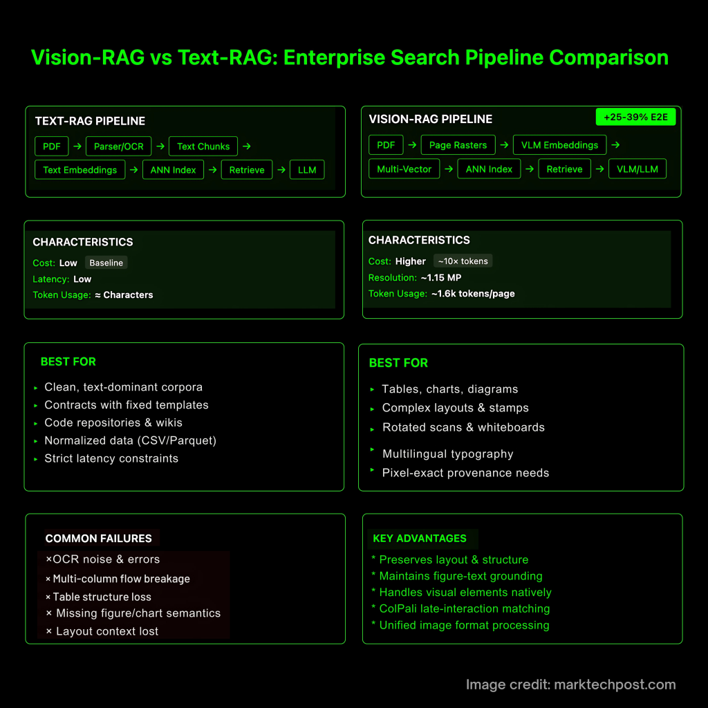
1. Align modalities across embeddings. Use encoders trained for textimage alignment (CLIP-family or VLM retrievers) and, in practice, dual-index: cheap text recall for coverage + vision rerank for precision. ColPali’s late-interaction (MaxSim-style) is a strong default for page images.
2. Feed high-fidelity inputs selectively. Coarse-to-fine: run BM25/DPR, take top-k pages to a vision reranker, then send only ROI crops (tables, charts, stamps) to the generator. This preserves crucial pixels without exploding tokens under tile-based accounting.
3. Engineer for real documents.
   • Tables: if you must parse, use table-structure models (e.g., PubTables-1M/TATR); otherwise prefer image-native retrieval.
   • Charts/diagrams: expect tick- and legend-level cues; resolution must retain these. Evaluate on chart-focused VQA sets.
   • Whiteboards/rotations/multilingual: page rendering avoids many OCR failure modes; multilingual scripts and rotated scans survive the pipeline.
   • Provenance: store page hashes and crop coordinates alongside embeddings to reproduce exact visual evidence used in answers.

Standard	Text-RAG	Vision-RAG
Ingest pipeline	PDF → parser/OCR → text chunks → text embeddings → ANN	PDF → page render(s) → VLM page/crop embeddings (often multi-vector, late interaction) → ANN. ColPali is a canonical implementation.
Primary failure modes	Parser drift, OCR noise, multi-column flow breakage, table structure loss, missing figure/chart semantics. Benchmarks exist because these errors are common.	Preserves layout/figures; failures shift to resolution/tiling choices and cross-modal alignment. VDocRAG formalizes “unified image” processing to avoid parsing loss.
Retriever representation	Single-vector text embeddings; rerank via lexical or cross-encoders	Page-image embeddings with late interaction (MaxSim-style) capture local regions; improves page-level retrieval on ViDoRe.
End-to-end gains (vs Text-RAG)	Baseline	+25–39% E2E on multimodal docs when both retrieval and generation are VLM-based (VisRAG).
Where it excels	Clean, text-dominant corpora; low latency/cost	Visually rich/structured docs: tables, charts, stamps, rotated scans, multilingual typography; unified page context helps QA.
Resolution sensitivity	Not applicable beyond OCR settings	Reasoning quality tracks input fidelity (ticks, small fonts). High-res document VLMs (e.g., Qwen2-VL family) emphasize this.
Cost model (inputs)	Tokens ≈ characters; cheap retrieval contexts	Image tokens grow with tiling: e.g., OpenAI base+tiles formula; Anthropic guidance ~1.15 MP ≈ ~1.6k tokens. Even when per-token price is equal (Gemini 2.5 Flash-Lite), high-res pages consume far more tokens.
Cross-modal alignment need	Not required	Critical: textimage encoders must share geometry for mixed queries; ColPali/ViDoRe demonstrate effective page-image retrieval aligned to language tasks.
Benchmarks to track	DocVQA (doc QA), PubTables-1M (table structure) for parsing-loss diagnostics.	ViDoRe (page retrieval), VisRAG (pipeline), VDocRAG (unified-image RAG).
Evaluation approach	IR metrics plus text QA; may miss figure-text grounding issues	Joint retrieval+gen on visually rich suites (e.g., OpenDocVQA under VDocRAG) to capture crop relevance and layout grounding.
Operational pattern	One-stage retrieval; cheap to scale	Coarse-to-fine: text recall → vision rerank → ROI crops to generator; keeps token costs bounded while preserving fidelity. (Tiling math/pricing inform budgets.)
When to prefer	Contracts/templates, code/wikis, normalized tabular data (CSV/Parquet)	Real-world enterprise docs with heavy layout/graphics; compliance workflows needing pixel-exact provenance (page hash + crop coords).
Representative systems	DPR/BM25 + cross-encoder rerank	ColPali (ICLR’25) vision retriever; VisRAG pipeline; VDocRAG unified image framework.

When Text-RAG is still the right default?

• Clean, text-dominant corpora (contracts with fixed templates, wikis, code)
• Strict latency/cost constraints for short answers
• Data already normalized (CSV/Parquet)—skip pixels and query the table store

Evaluation: measure retrieval + generation jointly

Add multimodal RAG benchmarks to your harness—e.g., M²RAG (multi-modal QA, captioning, fact-verification, reranking), REAL-MM-RAG (real-world multi-modal retrieval), and RAG-Check (relevance + correctness metrics for multi-modal context). These catch failure cases (irrelevant crops, figure-text mismatch) that text-only metrics miss.

Summary

Text-RAG remains efficient for clean, text-only data. Vision-RAG is the practical default for enterprise documents with layout, tables, charts, stamps, scans, and multilingual typography. Teams that (1) align modalities, (2) deliver selective high-fidelity visual evidence, and (3) evaluate with multimodal benchmarks consistently get higher retrieval precision and better downstream answers—now backed by ColPali (ICLR 2025), VisRAG’s 25–39% E2E lift, and VDocRAG’s unified image-format results.

References:

• ()
• ()

The post appeared first on .

In this tutorial, we explore advanced computer vision techniques using TorchVision’s v2 transforms, modern augmentation strategies, and powerful training enhancements. We walk through the process of building an augmentation pipeline, applying MixUp and CutMix, designing a modern CNN with attention, and implementing a robust training loop. By running everything seamlessly in Google Colab, we position ourselves to understand and apply state-of-the-art practices in deep learning with clarity and efficiency. Check out the .

!pip install torch torchvision torchaudio --quiet
!pip install matplotlib pillow numpy --quiet


import torch
import torchvision
from torchvision import transforms as T
from torchvision.transforms import v2
import torch.nn as nn
import torch.optim as optim
from torch.utils.data import DataLoader
import matplotlib.pyplot as plt
import numpy as np
from PIL import Image
import requests
from io import BytesIO


print(f"PyTorch version: {torch.__version__}")
print(f"TorchVision version: {torchvision.__version__}")

We begin by installing the libraries and importing all the essential modules for our workflow. We set up PyTorch, TorchVision v2 transforms, and supporting tools like NumPy, PIL, and Matplotlib, so we are ready to build and test advanced computer vision pipelines. Check out the .

class AdvancedAugmentationPipeline:
   def __init__(self, image_size=224, training=True):
       self.image_size = image_size
       self.training = training
       base_transforms = [
           v2.ToImage(),
           v2.ToDtype(torch.uint8, scale=True),
       ]
       if training:
           self.transform = v2.Compose([
               *base_transforms,
               v2.Resize((image_size + 32, image_size + 32)),
               v2.RandomResizedCrop(image_size, scale=(0.8, 1.0), ratio=(0.9, 1.1)),
               v2.RandomHorizontalFlip(p=0.5),
               v2.RandomRotation(degrees=15),
               v2.ColorJitter(brights=0.4, contst=0.4, sation=0.4, hue=0.1),
               v2.RandomGrayscale(p=0.1),
               v2.GaussianBlur(kernel_size=3, sigma=(0.1, 2.0)),
               v2.RandomPerspective(distortion_scale=0.1, p=0.3),
               v2.RandomAffine(degrees=10, translate=(0.1, 0.1), scale=(0.9, 1.1)),
               v2.ToDtype(torch.float32, scale=True),
               v2.Normalize(mean=[0.485, 0.456, 0.406], std=[0.229, 0.224, 0.225])
           ])
       else:
           self.transform = v2.Compose([
               *base_transforms,
               v2.Resize((image_size, image_size)),
               v2.ToDtype(torch.float32, scale=True),
               v2.Normalize(mean=[0.485, 0.456, 0.406], std=[0.229, 0.224, 0.225])
           ])
   def __call__(self, image):
       return self.transform(image)

We define an advanced augmentation pipeline that adapts to both training and validation modes. We apply powerful TorchVision v2 transforms, such as cropping, flipping, color jittering, blurring, perspective, and affine transformations, during training, while keeping validation preprocessing simple with resizing and normalization. This way, we ensure that we enrich the training data for better generalization while maintaining consistent and stable evaluation. Check out the .

class AdvancedMixupCutmix:
   def __init__(self, mixup_alpha=1.0, cutmix_alpha=1.0, prob=0.5):
       self.mixup_alpha = mixup_alpha
       self.cutmix_alpha = cutmix_alpha
       self.prob = prob
   def mixup(self, x, y):
       batch_size = x.size(0)
       lam = np.random.beta(self.mixup_alpha, self.mixup_alpha) if self.mixup_alpha > 0 else 1
       index = torch.randperm(batch_size)
       mixed_x = lam * x + (1 - lam) * x[index, :]
       y_a, y_b = y, y[index]
       return mixed_x, y_a, y_b, lam
   def cutmix(self, x, y):
       batch_size = x.size(0)
       lam = np.random.beta(self.cutmix_alpha, self.cutmix_alpha) if self.cutmix_alpha > 0 else 1
       index = torch.randperm(batch_size)
       y_a, y_b = y, y[index]
       bbx1, bby1, bbx2, bby2 = self._rand_bbox(x.size(), lam)
       x[:, :, bbx1:bbx2, bby1:bby2] = x[index, :, bbx1:bbx2, bby1:bby2]
       lam = 1 - ((bbx2 - bbx1) * (bby2 - bby1) / (x.size()[-1] * x.size()[-2]))
       return x, y_a, y_b, lam
   def _rand_bbox(self, size, lam):
       W = size[2]
       H = size[3]
       cut_rat = np.sqrt(1. - lam)
       cut_w = int(W * cut_rat)
       cut_h = int(H * cut_rat)
       cx = np.random.randint(W)
       cy = np.random.randint(H)
       bbx1 = np.clip(cx - cut_w // 2, 0, W)
       bby1 = np.clip(cy - cut_h // 2, 0, H)
       bbx2 = np.clip(cx + cut_w // 2, 0, W)
       bby2 = np.clip(cy + cut_h // 2, 0, H)
       return bbx1, bby1, bbx2, bby2
   def __call__(self, x, y):
       if np.random.random() > self.prob:
           return x, y, y, 1.0
       if np.random.random() < 0.5:
           return self.mixup(x, y)
       else:
           return self.cutmix(x, y)


class ModernCNN(nn.Module):
   def __init__(self, num_classes=10, dropout=0.3):
       super(ModernCNN, self).__init__()
       self.conv1 = self._conv_block(3, 64)
       self.conv2 = self._conv_block(64, 128, downsample=True)
       self.conv3 = self._conv_block(128, 256, downsample=True)
       self.conv4 = self._conv_block(256, 512, downsample=True)
       self.gap = nn.AdaptiveAvgPool2d(1)
       self.attention = nn.Sequential(
           nn.Linear(512, 256),
           nn.ReLU(),
           nn.Linear(256, 512),
           nn.Sigmoid()
       )
       self.classifier = nn.Sequential(
           nn.Dropout(dropout),
           nn.Linear(512, 256),
           nn.BatchNorm1d(256),
           nn.ReLU(),
           nn.Dropout(dropout/2),
           nn.Linear(256, num_classes)
       )
   def _conv_block(self, in_channels, out_channels, downsample=False):
       stride = 2 if downsample else 1
       return nn.Sequential(
           nn.Conv2d(in_channels, out_channels, 3, stride=stride, padding=1),
           nn.BatchNorm2d(out_channels),
           nn.ReLU(inplace=True),
           nn.Conv2d(out_channels, out_channels, 3, padding=1),
           nn.BatchNorm2d(out_channels),
           nn.ReLU(inplace=True)
       )
   def forward(self, x):
       x = self.conv1(x)
       x = self.conv2(x)
       x = self.conv3(x)
       x = self.conv4(x)
       x = self.gap(x)
       x = torch.flatten(x, 1)
       attention_weights = self.attention(x)
       x = x * attention_weights
       return self.classifier(x)

We strengthen our training with a unified MixUp/CutMix module, where we stochastically blend images or patch-swap regions and compute label interpolation with the exact pixel ratio. We pair this with a modern CNN that stacks progressive conv blocks, applies global average pooling, and uses a learned attention gate before a dropout-regularized classifier, so we improve generalization while keeping inference straightforward. Check out the .

class AdvancedTrainer:
   def __init__(self, model, device='cuda' if torch.cuda.is_available() else 'cpu'):
       self.model = model.to(device)
       self.device = device
       self.mixup_cutmix = AdvancedMixupCutmix()
       self.optimizer = optim.AdamW(model.parameters(), lr=1e-3, weight_decay=1e-4)
       self.scheduler = optim.lr_scheduler.OneCycleLR(
           self.optimizer, max_lr=1e-2, epochs=10, steps_per_epoch=100
       )
       self.criterion = nn.CrossEntropyLoss()
   def mixup_criterion(self, pred, y_a, y_b, lam):
       return lam * self.criterion(pred, y_a) + (1 - lam) * self.criterion(pred, y_b)
   def train_epoch(self, dataloader):
       self.model.train()
       total_loss = 0
       correct = 0
       total = 0
       for batch_idx, (data, target) in enumerate(dataloader):
           data, target = data.to(self.device), target.to(self.device)
           data, target_a, target_b, lam = self.mixup_cutmix(data, target)
           self.optimizer.zero_grad()
           output = self.model(data)
           if lam != 1.0:
               loss = self.mixup_criterion(output, target_a, target_b, lam)
           else:
               loss = self.criterion(output, target)
           loss.backward()
           torch.nn.utils.clip_grad_norm_(self.model.parameters(), max_norm=1.0)
           self.optimizer.step()
           self.scheduler.step()
           total_loss += loss.item()
           _, predicted = output.max(1)
           total += target.size(0)
           if lam != 1.0:
               correct += (lam * predicted.eq(target_a).sum().item() +
                          (1 - lam) * predicted.eq(target_b).sum().item())
           else:
               correct += predicted.eq(target).sum().item()
       return total_loss / len(dataloader), 100. * correct / total

We orchestrate training with AdamW, OneCycleLR, and dynamic MixUp/CutMix so we stabilize optimization and boost generalization. We compute an interpolated loss when mixing, clip gradients for safety, and step the scheduler each batch, so we track loss/accuracy per epoch in a single tight loop. Check out the .

def demo_advanced_techniques():
   batch_size = 16
   num_classes = 10
   sample_data = torch.randn(batch_size, 3, 224, 224)
   sample_labels = torch.randint(0, num_classes, (batch_size,))
   transform_pipeline = AdvancedAugmentationPipeline(training=True)
   model = ModernCNN(num_classes=num_classes)
   trainer = AdvancedTrainer(model)
   print(" Advanced Deep Learning Tutorial Demo")
   print("=" * 50)
   print("n1. Advanced Augmentation Pipeline:")
   augmented = transform_pipeline(Image.fromarray((sample_data[0].permute(1,2,0).numpy() * 255).astype(np.uint8)))
   print(f"   Original shape: {sample_data[0].shape}")
   print(f"   Augmented shape: {augmented.shape}")
   print(f"   Applied transforms: Resize, Crop, Flip, ColorJitter, Blur, Perspective, etc.")
   print("n2. MixUp/CutMix Augmentation:")
   mixup_cutmix = AdvancedMixupCutmix()
   mixed_data, target_a, target_b, lam = mixup_cutmix(sample_data, sample_labels)
   print(f"   Mixed batch shape: {mixed_data.shape}")
   print(f"   Lambda value: {lam:.3f}")
   print(f"   Technique: {'MixUp' if lam > 0.7 else 'CutMix'}")
   print("n3. Modern CNN Architecture:")
   model.eval()
   with torch.no_grad():
       output = model(sample_data)
   print(f"   Input shape: {sample_data.shape}")
   print(f"   Output shape: {output.shape}")
   print(f"   Features: Residual blocks, Attention, Global Average Pooling")
   print(f"   Parameters: {sum(p.numel() for p in model.parameters()):,}")
   print("n4. Advanced Training Simulation:")
   dummy_loader = [(sample_data, sample_labels)]
   loss, acc = trainer.train_epoch(dummy_loader)
   print(f"   Training loss: {loss:.4f}")
   print(f"   Training accuracy: {acc:.2f}%")
   print(f"   Learning rate: {trainer.scheduler.get_last_lr()[0]:.6f}")
   print("n Tutorial completed successfully!")
   print("This code demonstrates state-of-the-art techniques in deep learning:")
   print("• Advanced data augmentation with TorchVision v2")
   print("• MixUp and CutMix for better generalization")
   print("• Modern CNN architecture with attention")
   print("• Advanced training loop with OneCycleLR")
   print("• Gradient clipping and weight decay")


if __name__ == "__main__":
   demo_advanced_techniques()

We run a compact end-to-end demo where we visualize our augmentation pipeline, apply MixUp/CutMix, and double-check the ModernCNN with a forward pass. We then simulate one training epoch on dummy data to verify loss, accuracy, and learning-rate scheduling, so we confirm the full stack works before scaling to a real dataset.

In conclusion, we have successfully developed and tested a comprehensive workflow that integrates advanced augmentations, innovative CNN design, and modern training strategies. By experimenting with TorchVision v2, MixUp, CutMix, attention mechanisms, and OneCycleLR, we not only strengthen model performance but also deepen our understanding of cutting-edge techniques.

Check out the . Feel free to check out our . Also, feel free to follow us on  and don’t forget to join our  and Subscribe to .

The post appeared first on .

Alibaba has released Qwen3-Max, a trillion-parameter Mixture-of-Experts (MoE) model positioned as its most capable foundation model to date, with an immediate public on-ramp via Qwen Chat and Alibaba Cloud’s Model Studio API. The launch moves Qwen’s 2025 cadence from preview to production and centers on two variants: Qwen3-Max-Instruct for standard reasoning/coding tasks and Qwen3-Max-Thinking for tool-augmented “agentic” workflows.

What’s new at the model level?

• Scale & architecture: Qwen3-Max crosses the 1-trillion-parameter mark with an MoE design (sparse activation per token). Alibaba positions the model as its largest and most capable to date; public briefings and coverage consistently describe it as a 1T-parameter class system rather than another mid-scale refresh.
• Training/runtime posture: Qwen3-Max uses a sparse Mixture-of-Experts design and was pretrained on ~36T tokens (~2× Qwen2.5). The corpus skews toward multilingual, coding, and STEM/reasoning data. Post-training follows Qwen3’s four-stage recipe: long CoT cold-start → reasoning-focused RL → thinking/non-thinking fusion → general-domain RL. Alibaba confirms >1T parameters for Max; treat token counts/routing as team-reported until a formal Max tech report is published.
• Access: Qwen Chat showcases the general-purpose UX, while Model Studio exposes inference and “thinking mode” toggles (notably, incremental_output=true is required for Qwen3 thinking models). Model listings and pricing sit under Model Studio with regioned availability.

Benchmarks: coding, agentic control, math

• Coding (SWE-Bench Verified). Qwen3-Max-Instruct is reported at 69.6 on SWE-Bench Verified. That places it above some non-thinking baselines (e.g., DeepSeek V3.1 non-thinking) and slightly below Claude Opus 4 non-thinking in at least one roundup. Treat these as point-in-time numbers; SWE-Bench evaluations move quickly with harness updates.
• Agentic tool use (Tau2-Bench). Qwen3-Max posts 74.8 on Tau2-Bench—an agent/tool-calling evaluation—beating named peers in the same report. Tau2 is designed to test decision-making and tool routing, not just text accuracy, so gains here are meaningful for workflow automation.
• Math & advanced reasoning (AIME25, etc.). The Qwen3-Max-Thinking track (with tool use and a “heavy” runtime configuration) is described as near-perfect on key math benchmarks (e.g., AIME25) in multiple secondary sources and earlier preview coverage. Until an official technical report drops, treat “100%” claims as vendor-reported or community-replicated, not peer-reviewed.

Why two tracks—Instruct vs. Thinking?

Instruct targets conventional chat/coding/reasoning with tight latency, while Thinking enables longer deliberation traces and explicit tool calls (retrieval, code execution, browsing, evaluators), aimed at higher-reliability “agent” use cases. Critically, Alibaba’s API docs formalize the runtime switch: Qwen3 thinking models only operate with streaming incremental output enabled; commercial defaults are false, so callers must explicitly set it. This is a small but consequential contract detail if you’re instrumenting tools or chain-of-thought-like rollouts.

How to reason about the gains (signal vs. noise)?

• Coding: A 60–70 SWE-Bench Verified score range typically reflects non-trivial repository-level reasoning and patch synthesis under evaluation harness constraints (e.g., environment setup, flaky tests). If your workloads hinge on repo-scale code changes, these deltas matter more than single-file coding toys.
• Agentic: Tau2-Bench emphasizes multi-tool planning and action selection. Improvements here usually translate into fewer brittle hand-crafted policies in production agents, provided your tool APIs and execution sandboxes are robust.
• Math/verification: “Near-perfect” math numbers from heavy/thinky modes underscore the value of extended deliberation plus tools (calculators, validators). Portability of those gains to open-ended tasks depends on your evaluator design and guardrails.

Summary

Qwen3-Max is not a teaser—it’s a deployable 1T-parameter MoE with documented thinking-mode semantics and reproducible access paths (Qwen Chat, Model Studio). Treat day-one benchmark wins as directionally strong but continue local evals; the hard, verifiable facts are scale (≈36T tokens, >1T params) and the API contract for tool-augmented runs (incremental_output=true). For teams building coding and agentic systems, this is ready for hands-on trials and internal gating against SWE-/Tau2-style suites.

Check out the , and . Feel free to check out our . Also, feel free to follow us on  and don’t forget to join our  and Subscribe to .

The post appeared first on .