AI Tools & Reviews

xAI introduced , a cost-optimized successor to Grok-4 that merges “reasoning” and “non-reasoning” behaviors into a single set of weights controllable via system prompts. The model targets high-throughput search, coding, and Q&A with a 2M-token context window and native tool-use RL that decides when to browse the web, execute code, or call tools.

Architecture note

Previous Grok releases split long-chain “reasoning” and short “non-reasoning” responses across separate models. Grok-4-Fast’s unified weight space reduces end-to-end latency and tokens by steering behavior via system prompts, which is relevant for real-time applications (search, assistive agents, and interactive coding) where switching models penalizes both latency and cost.

Search and agentic use

Grok-4-Fast was trained end-to-end with tool-use reinforcement learning and shows gains on search-centric agent benchmarks: BrowseComp 44.9%, SimpleQA 95.0%, Reka Research 66.0%, plus higher scores on Chinese variants (e.g., BrowseComp-zh 51.2%). xAI also cites private battle-testing on LMArena where grok-4-fast-search (codename “menlo”) ranks #1 in the Search Arena with 1163 Elo, and the text variant (codename “tahoe”) sits at #8 in the Text Arena, roughly on par with grok-4-0709.

Performance and efficiency deltas

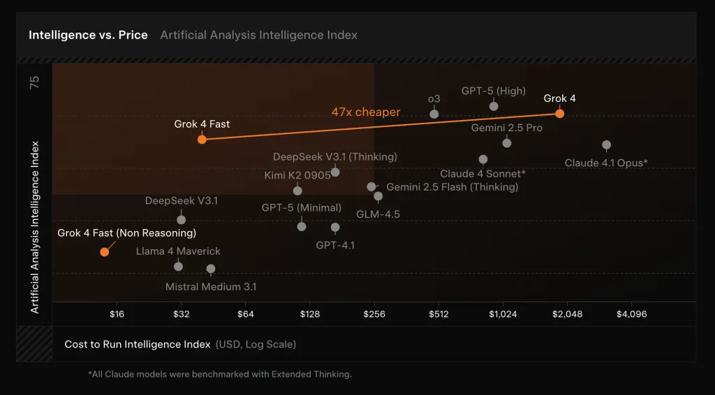
On internal and public benchmarks, Grok-4-Fast posts frontier-class scores while cutting token usage. xAI reports pass@1 results of 92.0% (AIME 2025, no tools), 93.3% (HMMT 2025, no tools), 85.7% (GPQA Diamond), and 80.0% (LiveCodeBench Jan–May), approaching or matching Grok-4 but using ~40% fewer “thinking” tokens on average. The company frames this as “intelligence density,” claiming a ~98% reduction in price to reach the same benchmark performance as Grok-4 when the lower token count and new per-token pricing are combined.

Deployment and price

The model is generally available to all users in Grok’s Fast and Auto modes across web and mobile; Auto will select Grok-4-Fast for difficult queries to improve latency without losing quality, and—for the first time—free users access xAI’s latest model tier. For developers, xAI exposes two SKUs—grok-4-fast-reasoning and grok-4-fast-non-reasoning—both with 2M context. Pricing (xAI API) is $0.20 / 1M input tokens (<128k), $0.40 / 1M input tokens (≥128k), $0.50 / 1M output tokens (<128k), $1.00 / 1M output tokens (≥128k), and $0.05 / 1M cached input tokens.

5 Technical Takeaways:

• Unified model + 2M context. Grok-4-Fast uses a single weight space for “reasoning” and “non-reasoning,” prompt-steered, with a 2,000,000-token window across both SKUs.
• Pricing for scale. API pricing starts at $0.20/M input, $0.50/M output, with cached input at $0.05/M and higher rates only beyond 128K context.
• Efficiency claims. xAI reports ~40% fewer “thinking” tokens at comparable accuracy vs Grok-4, yielding a ~98% lower price to match Grok-4 performance on frontier benchmarks.
• Benchmark profile. Reported pass@1: AIME-2025 92.0%, HMMT-2025 93.3%, GPQA-Diamond 85.7%, LiveCodeBench (Jan–May) 80.0%.
• Agentic/search use. Post-training with tool-use RL; positioned for browsing/search workflows with documented search-agent metrics and live-search billing in docs.

Summary

Grok-4-Fast packages Grok-4-level capability into a single, prompt-steerable model with a 2M-token window, tool-use RL, and pricing tuned for high-throughput search and agent workloads. Early public signals (LMArena #1 in Search, competitive Text placement) align with xAI’s claim of similar accuracy using ~40% fewer “thinking” tokens, translating to lower latency and unit cost in production.

Check out the . Feel free to check out our . Also, feel free to follow us on  and don’t forget to join our  and Subscribe to .

The post appeared first on .

Xiaomi’s MiMo team released MiMo-Audio, a 7-billion-parameter audio-language model that runs a single next-token objective over interleaved text and discretized speech, scaling pretraining beyond 100 million hours of audio.

What’s actually new?

Instead of relying on task-specific heads or lossy acoustic tokens, MiMo-Audio uses a bespoke RVQ (residual vector quantization) tokenizer that targets both semantic fidelity and high-quality reconstruction. The tokenizer runs at 25 Hz and outputs 8 RVQ layers (≈200 tokens/s), giving the LM access to “lossless” speech features it can model autoregressively alongside text.

Architecture: patch encoder → 7B LLM → patch decoder

To handle the audio/text rate mismatch, the system packs four timesteps per patch for LM consumption (downsampling 25 Hz → 6.25 Hz), then reconstructs full-rate RVQ streams with a causal patch decoder. A delayed multi-layer RVQ generation scheme staggers predictions per codebook to stabilize synthesis and respect inter-layer dependencies. All three parts—patch encoder, MiMo-7B backbone, and patch decoder—are trained under a single next-token objective.

Scale is the algorithm

Training proceeds in two big phases: (1) an “understanding” stage that optimizes text-token loss over interleaved speech-text corpora, and (2) a joint “understanding + generation” stage that turns on audio losses for speech continuation, S2T/T2S tasks, and instruction-style data. The report emphasizes a compute/data threshold where few-shot behavior appears to “switch on,” echoing emergence curves seen in large text-only LMs.

Benchmarks: speech intelligence and general audio

MiMo-Audio is evaluated on speech-reasoning suites (e.g., SpeechMMLU) and broad audio understanding benchmarks (e.g., MMAU), reporting strong scores across speech, sound, and music and a reduced “modality gap” between text-only and speech-in/speech-out settings. Xiaomi also releases MiMo-Audio-Eval, a public toolkit to reproduce these results. Listen-and-respond demos (speech continuation, voice/emotion conversion, denoising, and speech translation) are available online.

Why this is important?

The approach is intentionally simple—no multi-head task tower, no bespoke ASR/TTS objectives at pretraining time—just GPT-style next-token prediction over lossless audio tokens plus text. The key engineering ideas are (i) a tokenizer the LM can actually use without throwing away prosody and speaker identity; (ii) patchification to keep sequence lengths manageable; and (iii) delayed RVQ decoding to preserve quality at generation time. For teams building spoken agents, those design choices translate into few-shot speech-to-speech editing and robust speech continuation with minimal task-specific finetuning.

6 Technical Takeaways:

1. High-Fidelity Tokenization
   MiMo-Audio uses a custom RVQ tokenizer operating at 25 Hz with 8 active codebooks, ensuring speech tokens preserve prosody, timbre, and speaker identity while keeping them LM-friendly.
2. Patchified Sequence Modeling
   The model reduces sequence length by grouping 4 timesteps into one patch (25 Hz → 6.25 Hz), letting the 7B LLM handle long speech efficiently without discarding detail.
3. Unified Next-Token Objective
   Rather than separate heads for ASR, TTS, or dialogue, MiMo-Audio trains under a single next-token prediction loss across interleaved text and audio, simplifying architecture while supporting multi-task generalization.
4. Emergent Few-Shot Abilities
   Few-shot behaviors such as speech continuation, voice conversion, emotion transfer, and speech translation emerge once training surpasses a large-scale data threshold (~100M hours, trillions of tokens).
5. Benchmark Leadership
   MiMo-Audio sets state-of-the-art scores on SpeechMMLU (S2S 69.1, T2S 71.5) and MMAU (66.0 overall), while minimizing the text-to-speech modality gap to just 3.4 points.
6. Open Ecosystem Release
   Xiaomi provides the tokenizer, 7B checkpoints (base and instruct), MiMo-Audio-Eval toolkit, and public demos, enabling researchers and developers to test and extend speech-to-speech intelligence in open-source pipelines.

Summary

MiMo-Audio demonstrates that high-fidelity, RVQ-based “lossless” tokenization combined with patchified next-token pretraining at scale is sufficient to unlock few-shot speech intelligence without task-specific heads. The 7B stack—tokenizer → patch encoder → LLM → patch decoder—bridges the audio/text rate gap (25→6.25 Hz) and preserves prosody and speaker identity via delayed multi-layer RVQ decoding. 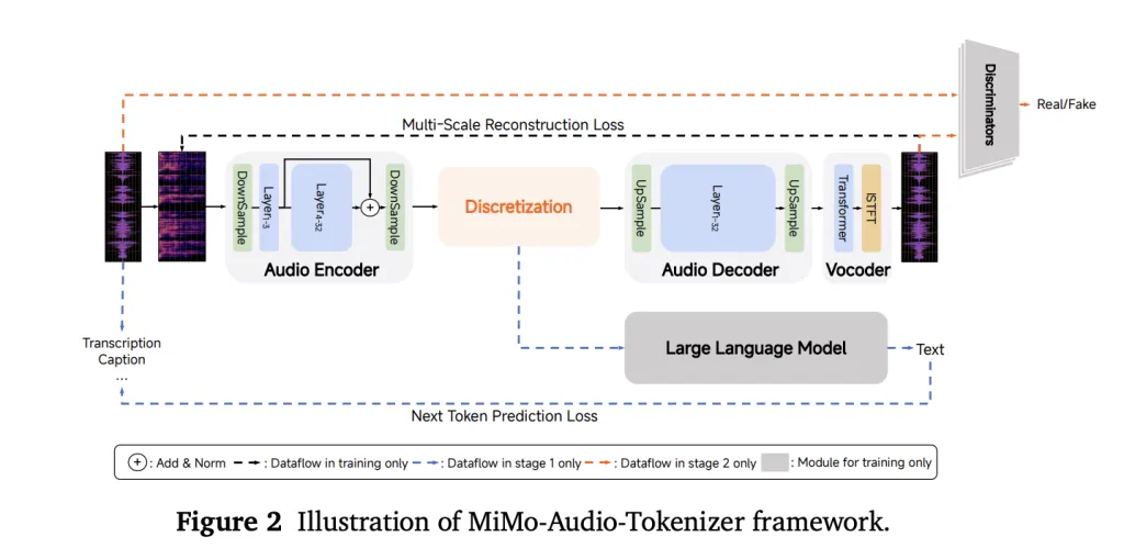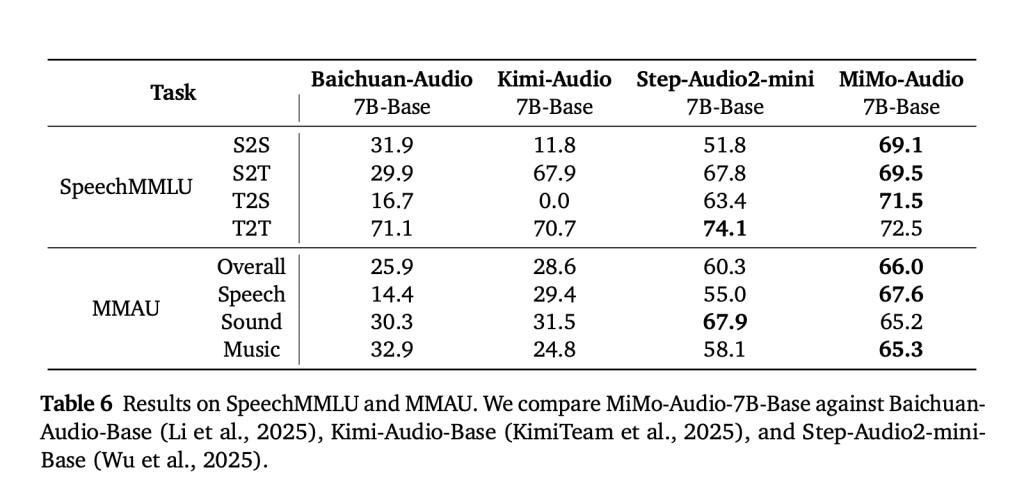Empirically, the model narrows the textspeech modality gap, generalizes across speech/sound/music benchmarks, and supports in-context S2S editing and continuation.

Check out the , and . Feel free to check out our . Also, feel free to follow us on  and don’t forget to join our  and Subscribe to .

The post appeared first on .

In this tutorial, we explore how we can seamlessly run MATLAB-style code inside Python by connecting Octave with the oct2py library. We set up the environment on Google Colab, exchange data between NumPy and Octave, write and call .m files, visualize plots generated in Octave within Python, and even work with toolboxes, structs, and .mat files. By doing this, we gain the flexibility of Python’s ecosystem while continuing to leverage the familiar syntax and numerical power of MATLAB/Octave in a single workflow. Check out the .

!apt-get -qq update
!apt-get -qq install -y octave gnuplot octave-signal octave-control > /dev/null
!python -m pip -q install oct2py scipy matplotlib pillow


from oct2py import Oct2Py, Oct2PyError
import numpy as np, matplotlib.pyplot as plt, textwrap
from scipy.io import savemat, loadmat
from PIL import Image


oc = Oct2Py()
print("Octave version:", oc.eval("version"))


def show_png(path, title=None):
   img = Image.open(path)
   plt.figure(figsize=(5,4)); plt.imshow(img); plt.axis("off")
   if title: plt.title(title)
   plt.show()

We begin by setting up Octave and essential libraries in Google Colab, ensuring that we have Octave-Forge packages and Python dependencies ready. We then initialize an Oct2Py session and define a helper function so we can display Octave-generated plots directly in our Python workflow. Check out the .

print("n--- Basic eval ---")
print(oc.eval("A = magic(4); A"))
print("eig(A) diag:", oc.eval("[V,D]=eig(A); diag(D)'"))
print("sin(pi/4):", oc.eval("sin(pi/4)"))


print("n--- NumPy exchange ---")
x = np.linspace(0, 2*np.pi, 100)
y = np.sin(x) + 0.1*np.random.randn(x.size)
y_filt = oc.feval("conv", y, np.ones(5)/5.0, "same") 
print("y_filt shape:", np.asarray(y_filt).shape)


print("n--- Cells & Structs ---")
cells = ["hello", 42, [1,2,3]]
oc.push("C", cells)
oc.eval("s = struct('name','Ada','score',99,'tags',{C});")
s = oc.pull("s")
print("Struct from Octave -> Python:", s)

We test the bridge between Python and Octave by running basic matrix operations, eigenvalue decomposition, and trigonometric evaluations directly in Octave. We then exchange NumPy arrays with Octave to perform a convolution filter and verify its shape. Finally, we demonstrate how to push Python lists into Octave as cell arrays, build a struct, and retrieve it back into Python for seamless data sharing. Check out the .

print("n--- Writing and calling .m files ---")
gd_code = r"""
function [w, hist] = gradient_descent(X, y, alpha, iters)
 % X: (n,m), y: (n,1). Adds bias; returns weights and loss history.
 if size(X,2) == 0, error('X must be 2D'); end
 n = rows(X);
 Xb = [ones(n,1), X];
 m = columns(Xb);
 w = zeros(m,1);
 hist = zeros(iters,1);
 for t=1:iters
   yhat = Xb*w;
   g = (Xb'*(yhat - y))/n;
   w = w - alpha * g;
   hist(t) = (sum((yhat - y).^2)/(2*n));
 endfor
endfunction
"""
with open("gradient_descent.m","w") as f: f.write(textwrap.dedent(gd_code))


np.random.seed(0)
X = np.random.randn(200, 3)
true_w = np.array([2.0, -1.0, 0.5, 3.0])    
y = true_w[0] + X @ true_w[1:] + 0.3*np.random.randn(200)
w_est, hist = oc.gradient_descent(X, y.reshape(-1,1), 0.1, 100, nout=2)
print("Estimated w:", np.ravel(w_est))
print("Final loss:", float(np.ravel(hist)[-1]))


print("n--- Octave plotting -> PNG -> Python display ---")
oc.eval("x = linspace(0,2*pi,400); y = sin(2*x) .* exp(-0.2*x);")
oc.eval("figure('visible','off'); plot(x,y,'linewidth',2); grid on; title('Damped Sine (Octave)');")
plot_path = "/content/oct_plot.png"
oc.eval(f"print('{plot_path}','-dpng'); close all;")
show_png(plot_path, title="Octave-generated Plot")

We write a custom gradient_descent.m in Octave, call it from Python with nout=2, and confirm that we recover reasonable weights and a decreasing loss. We then render a damped sine plot in an off-screen Octave figure and display the saved PNG inline in our Python notebook, keeping the whole workflow seamless. Check out the .

print("n--- Packages (signal/control) ---")
signal_ok = True
try:
   oc.eval("pkg load signal; pkg load control;")
   print("Loaded: signal, control")
except Oct2PyError as e:
   signal_ok = False
   print("Could not load signal/control, skipping package demo.nReason:", str(e).splitlines()[0])


if signal_ok:
   oc.push("t", np.linspace(0,1,800))
   oc.eval("x = sin(2*pi*5*t) + 0.5*sin(2*pi*40*t);")
   oc.eval("[b,a] = butter(4, 10/(800/2)); xf = filtfilt(b,a,x);")
   xf = oc.pull("xf")
   plt.figure(); plt.plot(xf); plt.title("Octave signal package: filtered"); plt.show()


print("n--- Function handles ---")
oc.eval("""
f = @(z) z.^2 + 3*z + 2;
vals = feval(f, [0 1 2 3]);
""")
vals = oc.pull("vals")
print("f([0,1,2,3]) =", np.ravel(vals))


quadfun_code = r"""
function y = quadfun(z)
 y = z.^2 + 3*z + 2;
end
"""
with open("quadfun.m","w") as f: f.write(textwrap.dedent(quadfun_code))
vals2 = oc.quadfun(np.array([0,1,2,3], dtype=float))
print("quadfun([0,1,2,3]) =", np.ravel(vals2))

We load the signal and control packages so we can design a Butterworth filter in Octave and visualize the filtered waveform back in Python. We also work with function handles by evaluating an anonymous quadratic inside Octave and, for robustness, define a named quadfun.m that we call from Python, showing both handle-based and file-based function calls in the same flow. Check out the .

print("n--- .mat I/O ---")
data_py = {"A": np.arange(9).reshape(3,3), "label": "demo"}
savemat("demo.mat", data_py)
oc.eval("load('demo.mat'); A2 = A + 1;")
oc.eval("save('-mat','demo_from_octave.mat','A2','label');")
back = loadmat("demo_from_octave.mat")
print("Keys from Octave-saved mat:", list(back.keys()))


print("n--- Error handling ---")
try:
   oc.eval("no_such_function(1,2,3);")
except Oct2PyError as e:
   print("Caught Octave error as Python exception:n", str(e).splitlines()[0])


print("n--- Simple Octave benchmark ---")
oc.eval("N = 2e6; a = rand(N,1);")


oc.eval("tic; s1 = sum(a); tv = toc;")
t_vec = float(oc.pull("tv"))


oc.eval("tic; s2 = 0; for i=1:length(a), s2 += a(i); end; tl = toc;")
t_loop = float(oc.pull("tl"))


print(f"Vectorized sum: {t_vec:.4f}s | Loop sum: {t_loop:.4f}s")


print("n--- Multi-file pipeline ---")
pipeline_m = r"""
function out = mini_pipeline(x, fs)
 try, pkg load signal; catch, end
 [b,a] = butter(6, 0.2);
 y = filtfilt(b,a,x);
 y_env = abs(hilbert(y));
 out = struct('rms', sqrt(mean(y.^2)), 'peak', max(abs(y)), 'env', y_env(1:10));
end
"""
with open("mini_pipeline.m","w") as f: f.write(textwrap.dedent(pipeline_m))


fs = 200.0
sig = np.sin(2*np.pi*3*np.linspace(0,3,int(3*fs))) + 0.1*np.random.randn(int(3*fs))
out = oc.mini_pipeline(sig, fs, nout=1)
print("mini_pipeline -> keys:", list(out.keys()))
print("RMS ~", float(out["rms"]), "| Peak ~", float(out["peak"]), "| env head:", np.ravel(out["env"])[:5])


print("nAll sections executed. You are now running MATLAB/Octave code from Python!")

We exchange .mat files between Python and Octave, confirming that data flows both ways without issues. We also test error handling by catching an Octave error as a Python exception. Next, we benchmark vectorized versus looped summations in Octave, showing the performance edge of vectorization. Finally, we built a multi-file pipeline that applies filtering and envelope detection, returning key statistics to Python, which demonstrates how we can organize Octave code into reusable components within our Python workflow.

In conclusion, we see how we can integrate Octave’s MATLAB-compatible features directly into Python and Colab. We successfully test data exchange, custom functions, plotting, package usage, and performance benchmarking, demonstrating that we can mix MATLAB/Octave workflows with Python without leaving our notebook. By combining the strengths of both environments, we put ourselves in a position to solve problems more efficiently and with greater flexibility.

Check out the . Feel free to check out our . Also, feel free to follow us on  and don’t forget to join our  and Subscribe to .

The post appeared first on .