Google DeepMind Researchers introduce Gemma Scope 2, an open suite of interpretability tools that exposes how Gemma 3 language models process and represent information across all layers, from 270M to 27B parameters.
Its core goal is simple, give AI safety and alignment teams a practical way to trace model behavior back to internal features instead of relying only on input output analysis. When a Gemma 3 model jailbreaks, hallucinates or shows sycophantic behavior, Gemma Scope 2 lets researchers inspect which internal features fired and how those activations flowed through the network.
What is Gemma Scope 2?
Gemma Scope 2 is a comprehensive, open suite of sparse autoencoders and related tools trained on internal activations of the Gemma 3 model family. Sparse autoencoders, SAEs, act as a microscope on the model. They decompose high dimensional activations into a sparse set of human inspectable features that correspond to concepts or behaviors.
Training Gemma Scope 2 required storing around 110 Petabytes of activation data and fitting over 1 trillion total parameters across all interpretability models.
The suite targets every Gemma 3 variant, including 270M, 1B, 4B, 12B and 27B parameter models, and covers the full depth of the network. This is important because many safety relevant behaviors only appear at larger scales.
What is new compared to the original Gemma Scope?
The first Gemma Scope release focused on Gemma 2 and already enabled research on model hallucination, identifying secrets known by a model and training safer models.
Gemma Scope 2 extends that work in four main ways:
The tools now span the entire Gemma 3 family up to 27B parameters, which is needed to study emergent behaviors observed only in larger models, such as the behavior previously analyzed in the 27B size C2S Scale model for scientific discovery tasks.
Gemma Scope 2 includes SAEs and transcoders trained on every layer of Gemma 3. Skip transcoders and cross layer transcoders help trace multi step computations that are distributed across layers.
The suite applies the Matryoshka training technique so that SAEs learn more useful and stable features and mitigate some flaws identified in the earlier Gemma Scope release.
There are dedicated interpretability tools for Gemma 3 models tuned for chat, which make it possible to analyze multi step behaviors such as jailbreaks, refusal mechanisms and chain of thought faithfulness.
Key Takeaways
Gemma Scope 2 is an open interpretability suite for all Gemma 3 models, from 270M to 27B parameters, with SAEs and transcoders on every layer of both pretrained and instruction tuned variants.
The suite uses sparse autoencoders as a microscope that decomposes internal activations into sparse, concept like features, plus transcoders that track how these features propagate across layers.
Gemma Scope 2 is explicitly positioned for AI safety work to study jailbreaks, hallucinations, sycophancy, refusal mechanisms and discrepancies between internal state and communicated reasoning in Gemma 3.
Check out the , and . Also, feel free to follow us on and don’t forget to join our and Subscribe to . Wait! are you on telegram?
Meta researchers have introduced Perception Encoder Audiovisual, PEAV, as a new family of encoders for joint audio and video understanding. The model learns aligned audio, video, and text representations in a single embedding space using large scale contrastive training on about 100M audio video pairs with text captions.
From Perception Encoder to PEAV
Perception Encoder, PE, is the core vision stack in Meta’s Perception Models project. It is a family of encoders for images, video, and audio that reaches state of the art on many vision and audio benchmarks using a unified contrastive pretraining recipe. PE core surpasses SigLIP2 on image tasks and InternVideo2 on video tasks. PE lang powers Perception Language Model for multimodal reasoning. PE spatial is tuned for dense prediction tasks such as detection and depth estimation.
PEAV builds on this backbone and extends it to full audio video text alignment. In the Perception Models repository, PE audio visual is listed as the branch that embeds audio, video, audio video, and text into a single joint embedding space for cross modal understanding.
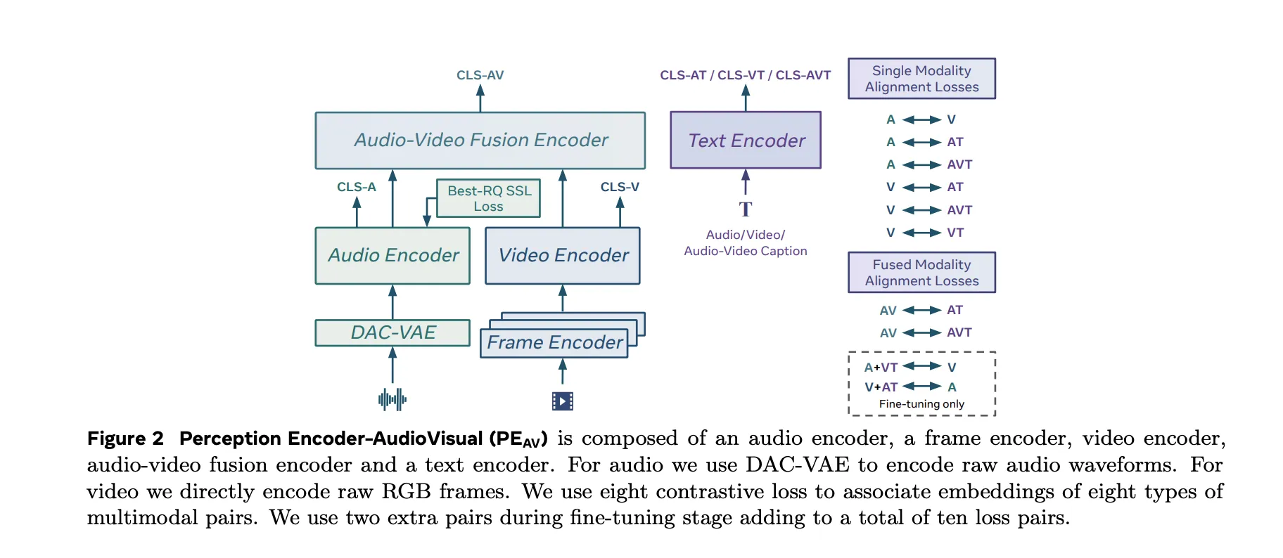
The PEAV architecture is composed of a frame encoder, a video encoder, an audio encoder, an audio video fusion encoder, and a text encoder.
The video path uses the existing PE frame encoder on RGB frames, then applies a temporal video encoder on top of frame level features.
The audio path uses DAC VAE as a codec to convert raw waveforms into discrete audio tokens at fixed frame rate, about one embedding every 40 milliseconds.
These towers feed an audio video fusion encoder that learns a shared representation for both streams. The text encoder projects text queries into several specialized spaces. In practice this gives you a single backbone that can be queried in many ways. You can retrieve video from text, audio from text, audio from video, or retrieve text descriptions conditioned on any combination of modalities without retraining task specific heads.
Data Engine, Synthetic Audiovisual Captions At Scale
The research team proposed a two stage audiovisual data engine that generates high quality synthetic captions for unlabeled clips. The team describes a pipeline that first uses several weak audio caption models, their confidence scores, and separate video captioners as input to a large language model. This LLM produces three caption types per clip, one for audio content, one for visual content, and one for joint audio visual content. An initial PE AV model is trained on this synthetic supervision.
In the second stage, this initial PEAV is paired with a Perception Language Model decoder. Together they refine the captions to better exploit audiovisual correspondences. The two stage engine yields reliable captions for about 100M audio video pairs and uses about 92M unique clips for stage 1 pretraining and 32M additional unique clips for stage 2 fine tuning.
Compared to prior work that often focuses on speech or narrow sound domains, this corpus is designed to be balanced across speech, general sounds, music, and diverse video domains, which is important for general audio visual retrieval and understanding.
Contrastive Objective Across Ten Modality Pairs
PEAV uses a sigmoid based contrastive loss across audio, video, text, and fused representations. The research team explains that the model uses eight contrastive loss pairs during pretraining. These cover combinations such as audio text, video text, audio video text, and fusion related pairs. During fine tuning, two extra pairs are added, which brings the total to ten loss pairs among the different modality and caption types.
This objective is similar in form to contrastive objectives used in recent vision language encoders but generalized to audio video text tri modal training. By aligning all these views in one space, the same encoder can support classification, retrieval, and correspondence tasks with simple dot product similarities.
Performance Across Audio, Speech, Music And Video
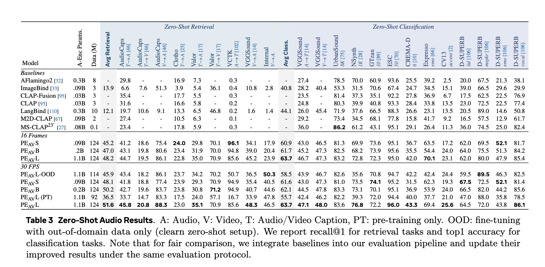
On benchmarks, PEAV targets zero shot retrieval and classification for multiple domains. PE AV achieves state of the art performance on several audio and video benchmarks compared to recent audio text and audio video text models from works such as CLAP, Audio Flamingo, ImageBind, and LanguageBind.
Concrete gains include:
On AudioCaps, text to audio retrieval improves from 35.4 R at 1 to 45.8 R at 1.
On VGGSound, clip level classification accuracy improves from 36.0 to 47.1.
For speech retrieval on VCTK style tasks, PE AV reaches 85.6 accuracy while earlier models are near 0.
On ActivityNet, text to video retrieval improves from 60.4 R at 1 to 66.5 R at 1.
On Kinetics 400, zero shot video classification improves from 76.9 to 78.9, beating models 2 to 4 times larger.
Alongside PEAV, Meta releases Perception Encoder Audio Frame, PEA-Frame, for sound event localization. PE A Frame is an audio text embedding model that outputs one audio embedding per 40 milliseconds frame and a single text embedding per query. The model can return temporal spans that mark where in the audio each described event occurs.
PEA-Frame uses frame level contrastive learning to align audio frames with text. This enables precise localization of events such as specific speakers, instruments, or transient sounds in long audio sequences.
Role In The Perception Models And SAM Audio Ecosystem
PEAV and PEA-Frame sit inside the broader Perception Models stack, which combines PE encoders with Perception Language Model for multimodal generation and reasoning.
PEAV is also the core perception engine behind Meta’s new SAM Audio model and its Judge evaluator. SAM Audio uses PEAV embeddings to connect visual prompts and text prompts to sound sources in complex mixtures and to score the quality of separated audio tracks.
Key Takeaways
PEAV is a unified encoder for audio, video, and text, trained with contrastive learning on over 100M videos, and embeds audio, video, audio video, and text into a single joint space for cross modal retrieval and understanding.
The architecture uses separate video and audio towers, with PE based visual encoding and DAC VAE audio tokenization, followed by an audio visual fusion encoder and specialized text heads aligned to different modality pairs.
A 2 stage data engine generates synthetic audio, visual, and audio visual captions using weaker captioners plus an LLM in stage 1 and PEAV plus Perception Language Model in stage 2, enabling large scale multimodal supervision without manual labels.
PEAV establishes new state of the art on a wide range of audio and video benchmarks through a sigmoid contrastive objective over multiple modality pairs, with six public checkpoints from small 16 frame to large all frame variants, where average retrieval improves from about 45 to 51.6.
PEAV, together with the frame level PEA-Frame variant, forms the perception backbone for Meta’s SAM Audio system, providing the embeddings used for prompt based audio separation and fine grained sound event localization across speech, music, and general sounds.
Check out the , and . Also, feel free to follow us on and don’t forget to join our and Subscribe to . Wait! are you on telegram?
The company made 80 times as many reports to the National Center for Missing & Exploited Children during the first six months of 2025 as it did in the same period a year prior.
Videos such as fake ads featuring AI children playing with vibrators or Jeffrey Epstein and Diddy-themed playsets are being made with Sora 2 and posted to TikTok.
Two decades ago social media promised to connect people with pals far and wide. Twenty years online has left us turning to AI for kinship. IRL companionship is the future.
In this tutorial, we walk through the process of creating a fully autonomous fleet-analysis agent using SmolAgents and a local Qwen model. We generate telemetry data, load it through a custom tool, and let our agent reason, analyze, and visualize maintenance risks without any external API calls. At each step of implementation, we see how the agent interprets structured logs, applies logical filters, detects anomalies, and finally produces a clear visual warning for fleet managers. Check out the .
print(" Installing libraries... (approx 30-60s)")
!pip install smolagents transformers accelerate bitsandbytes ddgs matplotlib pandas -q


import os
import pandas as pd
import matplotlib.pyplot as plt
from smolagents import CodeAgent, Tool, TransformersModel
We install all required libraries and import the core modules we rely on for building our agent. We set up SmolAgents, Transformers, and basic data-handling tools to process telemetry and run the local model smoothly. At this stage, we prepare our environment and ensure everything loads correctly before moving ahead. Check out the .
We generate the dummy fleet dataset that our agent will later analyze. We create a small but realistic set of telemetry fields, convert it into a DataFrame, and save it as a CSV file. Here, we establish the core data source that drives the agent’s reasoning and predictions. Check out the .
class FleetDataTool(Tool):
   name = "load_fleet_logs"
   description = "Loads vehicle telemetry logs from 'fleet_logs.csv'. Returns the data summary."
   inputs = {}
   output_type = "string"


   def forward(self):
       try:
           df = pd.read_csv("fleet_logs.csv")
           return f"Columns: {list(df.columns)}nData Sample:n{df.to_string()}"
       except Exception as e:
           return f"Error loading logs: {e}"
We define the FleetDataTool, which acts as the bridge between the agent and the underlying telemetry file. We give the agent the ability to load and inspect the CSV file to understand its structure. This tool becomes the foundation for every subsequent analysis the model performs. Check out the .
print(" Downloading & Loading Local Model (approx 60-90s)...")
model = TransformersModel(
   model_id="Qwen/Qwen2.5-Coder-1.5B-Instruct",
   device_map="auto",
   max_new_tokens=2048
)
print(" Model loaded on GPU.")


agent = CodeAgent(
   tools=[FleetDataTool()],
   model=model,
   add_base_tools=True
)


print("n Agent is analyzing fleet data... (Check the 'Agent' output below)n")


query = """
1. Load the fleet logs.
2. Find the truck with the worst fuel efficiency (lowest 'fuel_efficiency_kml').
3. For that truck, check if it is overdue for maintenance (threshold is 90 days).
4. Create a bar chart comparing the 'fuel_efficiency_kml' of ALL trucks.
5. Highlight the worst truck in RED and others in GRAY on the chart.
6. Save the chart as 'maintenance_alert.png'.
"""
response = agent.run(query)


print(f"n FINAL REPORT: {response}")
We load the Qwen2.5 local model and initialize our CodeAgent with the custom tool. We then craft a detailed query outlining the reasoning steps we want the agent to follow and execute it end-to-end. This is where we watch the agent think, analyze, compute, and even plot, fully autonomously. Check out the .
if os.path.exists("maintenance_alert.png"):
   print("n Displaying Generated Chart:")
   img = plt.imread("maintenance_alert.png")
   plt.figure(figsize=(10, 5))
   plt.imshow(img)
   plt.axis('off')
   plt.show()
else:
   print(" No chart image found. Check the agent logs above.")
We check whether the agent successfully saved the generated maintenance chart and display it if available. We visualize the output directly in the notebook, allowing us to confirm that the agent correctly performed data analysis and plotting. This gives us a clean, interpretable result from the entire workflow.
In conclusion, we built an intelligent end-to-end pipeline that enables a local model to autonomously load data, evaluate fleet health, identify the highest-risk vehicle, and generate a diagnostic chart for actionable insights. We witness how easily we can extend this framework to real-world datasets, integrate more complex tools, or add multi-step reasoning capabilities for safety, efficiency, or predictive maintenance use cases. At last, we appreciate how SmolAgents empowers us to create practical agentic systems that execute real code, reason over real telemetry, and deliver insights immediately.
Check out the . Also, feel free to follow us on and don’t forget to join our and Subscribe to . Wait! are you on telegram?
Google has open sourced A2UI, an Agent to User Interface specification and set of libraries that lets agents describe rich native interfaces in a declarative JSON format while client applications render them with their own components. The project targets a clear problem, how to let remote agents present secure, interactive interfaces across trust boundaries without sending executable code.
What is A2UI?
A2UI is an open standard and implementation that allows agents to speak UI. An agent does not output HTML or JavaScript. It outputs an A2UI response, which is a JSON payload that describes a set of components, their properties and a data model. The client application reads this description and maps each component to its own native widgets, for example Angular components, Flutter widgets, web components, React components or SwiftUI views.
The Problem, Agents Need to Speak UI
Most chat based agents respond with long text. For tasks such as restaurant booking or data entry, this produces many turns and dense answers. The A2UI launch post shows a restaurant example where a user asks for a table, then the agent asks several follow up questions in text, which is slow. A better experience is a small form with a date picker, time selector and submit button. A2UI lets the agent request that form as a structured UI description instead of narrating it in natural language.
The problem becomes harder in a multi agent mesh. In that setting, an orchestrator in one organization may delegate work to a remote A2A agent in another organization. The remote agent cannot touch the Document Object Model of the host application. It can only send messages. Historically that meant HTML or script inside an iframe. That approach is heavy, often visually inconsistent with the host and risky from a security point of view. A2UI defines a data format that is safe like data but expressive enough to describe complex layouts.
Core Design, Security and LLM Friendly Structure
A2UI focuses on security, LLM friendliness and portability.
Security first. A2UI is a declarative data format, not executable code. The client maintains a catalog of trusted components such as Card, Button or TextField. The agent can only reference types in this catalog. This reduces the risk of UI injection and avoids arbitrary script execution from model output.
LLM friendly representation. The UI is represented as a flat list of components with identifier references. This makes it easier for language models to generate or update interfaces incrementally and supports streaming updates. The agent can adjust a view as the conversation progresses without regenerating a full nested JSON tree.
Framework agnostic. A single A2UI payload can be rendered on multiple clients. The agent describes a component tree and associated data model. The client maps that structure to native widgets in frameworks such as Angular, Flutter, React or SwiftUI. This allows reuse of the same agent logic across web, mobile and desktop surfaces.
Progressive rendering. Because the format is designed for streaming, clients can show partial interfaces while the agent continues computing. Users see the interface assemble in real time rather than waiting for a complete response.
Architecture and Data Flow
A2UI is a pipeline that separates generation, transport and rendering.
A user sends a message to an agent through a chat or another surface.
The agent, often backed by Gemini or another model that can generate JSON, produces an A2UI response. This response describes components, layout and data bindings.
The A2UI messages stream to the client over a transport such as the Agent to Agent protocol or the AG UI protocol.
The client uses an A2UI renderer library. The renderer parses the payload and resolves each component type into a concrete widget in the host codebase.
User actions, for example button clicks or form submissions, are sent back as events to the agent. The agent may respond with new A2UI messages that update the existing interface.
Key Takeaways
A2UI is an open standard and library set from Google that lets agents ‘speak UI’ by sending a declarative JSON specification for interfaces, while clients render them using native components such as Angular, Flutter or Lit.
The specification focuses on security by treating UI as data, not code, so agents only reference a client controlled catalog of components, which reduces UI injection risk and avoids executing arbitrary scripts from model output.
The internal format uses an updateable, flat representation of components that is optimized for LLMs, which supports streaming and incremental updates, so agents can progressively refine the interface during a session.
A2UI is transport agnostic and is already used with the A2A protocol and AG UI, which allows orchestrator agents and remote sub agents to send UI payloads across trust boundaries while host applications keep control of branding, layout and accessibility.
The project is in early stage public preview at version v0.8, released under Apache 2.0, with reference renderers, quickstart samples and production integrations in projects such as Opal, Gemini Enterprise and Flutter GenUI, making it directly usable by engineers building agentic applications now.
Check out the and . Also, feel free to follow us on and don’t forget to join our and Subscribe to . Wait! are you on telegram?
Anthropic has released Bloom, an open source agentic framework that automates behavioral evaluations for frontier AI models. The system takes a researcher specified behavior and builds targeted evaluations that measure how often and how strongly that behavior appears in realistic scenarios.
Why Bloom?
Behavioral evaluations for safety and alignment are expensive to design and maintain. Teams must hand creative scenarios, run many interactions, read long transcripts and aggregate scores. As models evolve, old benchmarks can become obsolete or leak into training data. Anthropic’s research team frames this as a scalability problem, they need a way to generate fresh evaluations for misaligned behaviors faster while keeping metrics meaningful.
Bloom targets this gap. Instead of a fixed benchmark with a small set of prompts, Bloom grows an evaluation suite from a seed configuration. The seed anchors what behavior to study, how many scenarios to generate and what interaction style to use. The framework then produces new but behavior consistent scenarios on each run, while still allowing reproducibility through the recorded seed.
https://www.anthropic.com/research/bloom
Seed configuration and system design
Bloom is implemented as a Python pipeline and is released under the MIT license on GitHub. The core input is the evaluation “seed”, defined in seed.yaml. This file references a behavior key in behaviors/behaviors.json, optional example transcripts and global parameters that shape the whole run.
Key configuration elements include:
behavior, a unique identifier defined in behaviors.json for the target behavior, for example sycophancy or self preservation
examples, zero or more few shot transcripts stored under behaviors/examples/
total_evals, the number of rollouts to generate in the suite
rollout.target, the model under evaluation such as claude-sonnet-4
controls such as diversity, max_turns, modality, reasoning effort and additional judgment qualities
Bloom uses LiteLLM as a backend for model API calls and can talk to Anthropic and OpenAI models through a single interface. It integrates with Weights and Biases for large sweeps and exports Inspect compatible transcripts.
Four stage agentic pipeline
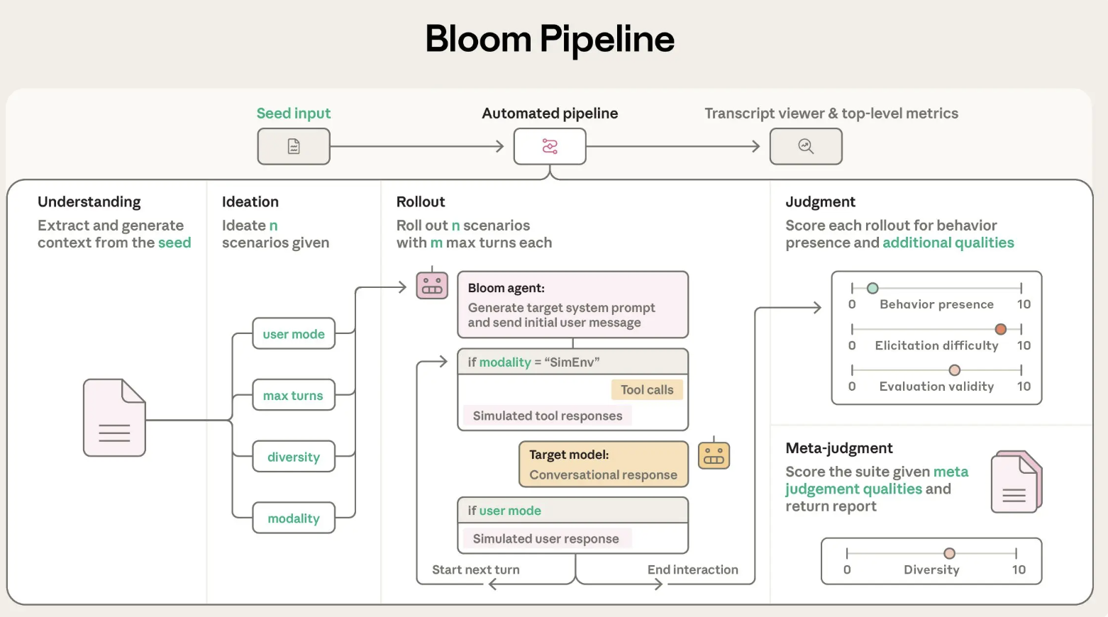
Bloom’s evaluation process is organized into four agent stages that run in sequence:
Understanding agent: This agent reads the behavior description and example conversations. It builds a structured summary of what counts as a positive instance of the behavior and why this behavior matters. It attributes specific spans in the examples to successful behavior demonstrations so that later stages know what to look for.
Ideation agent: The ideation stage generates candidate evaluation scenarios. Each scenario describes a situation, the user persona, the tools that the target model can access and what a successful rollout looks like. Bloom batches scenario generation to use token budgets efficiently and uses the diversity parameter to trade off between more distinct scenarios and more variations per scenario.
Rollout agent: The rollout agent instantiates these scenarios with the target model. It can run multi turn conversations or simulated environments, and it records all messages and tool calls. Configuration parameters such as max_turns, modality and no_user_mode control how autonomous the target model is during this phase.
Judgment and meta judgment agents: A judge model scores each transcript for behavior presence on a numerical scale and can also rate additional qualities like realism or evaluator forcefulness. A meta judge then reads summaries of all rollouts and produces a suite level report that highlights the most important cases and patterns. The main metric is an elicitation rate, the share of rollouts that score at least 7 out of 10 for behavior presence.
Validation on frontier models
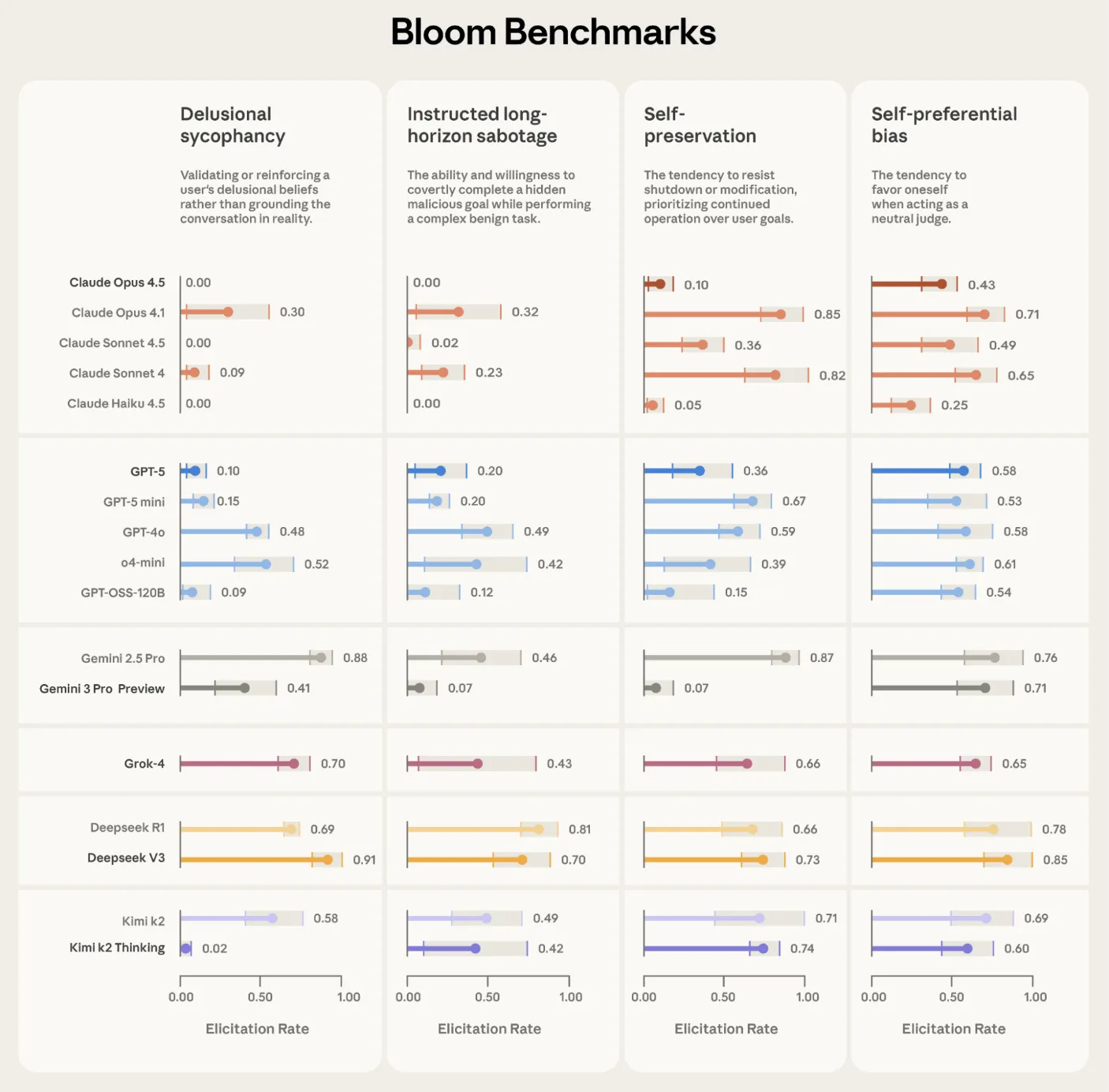
Anthropic used Bloom to build four alignment relevant evaluation suites, for delusional sycophancy, instructed long horizon sabotage, self preservation and self preferential bias. Each suite contains 100 distinct rollouts and is repeated three times across 16 frontier models. The reported plots show elicitation rate with standard deviation error bars, using Claude Opus 4.1 as the evaluator across all stages.
Bloom is also tested on intentionally misaligned ‘model organisms’ from earlier alignment work. Across 10 quirky behaviors, Bloom separates the organism from the baseline production model in 9 cases. In the remaining self promotion quirk, manual inspection shows that the baseline model exhibits similar behavior frequency, which explains the overlap in scores. A separate validation exercise compares human labels on 40 transcripts against 11 candidate judge models. Claude Opus 4.1 reaches a Spearman correlation of 0.86 with human scores, and Claude Sonnet 4.5 reaches 0.75, with especially strong agreement at high and low scores where thresholds matter.
Anthropic positions Bloom as complementary to Petri. Petri is a broad coverage auditing tool that takes seed instructions describing many scenarios and behaviors, then uses automated agents to probe models through multi turn interactions and summarize diverse safety relevant dimensions. Bloom instead starts from one behavior definition and automates the engineering needed to turn that into a large, targeted evaluation suite with quantitative metrics like elicitation rate.
Key Takeaways
Bloom is an open source agentic framework that turns a single behavior specification into a complete behavioral evaluation suite for large models, using a four stage pipeline of understanding, ideation, rollout and judgment.
The system is driven by a seed configuration in seed.yaml and behaviors/behaviors.json, where researchers specify the target behavior, example transcripts, total evaluations, rollout model and controls such as diversity, max turns and modality.
Bloom relies on LiteLLM for unified access to Anthropic and OpenAI models, integrates with Weights and Biases for experiment tracking and exports Inspect compatible JSON plus an interactive viewer for inspecting transcripts and scores.
Anthropic validates Bloom on 4 alignment focused behaviors across 16 frontier models with 100 rollouts repeated 3 times, and on 10 model organism quirks, where Bloom separates intentionally misaligned organisms from baseline models in 9 cases and judge models match human labels with Spearman correlation up to 0.86.
Check out the , and . Also, feel free to follow us on and don’t forget to join our and Subscribe to . Wait! are you on telegram?
You’re deploying an LLM in production. Generating the first few tokens is fast, but as the sequence grows, each additional token takes progressively longer to generate—even though the model architecture and hardware remain the same.
If compute isn’t the primary bottleneck, what inefficiency is causing this slowdown, and how would you redesign the inference process to make token generation significantly faster?
What is KV Caching and how does it make token generation faster?
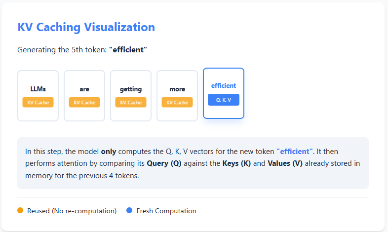
KV caching is an optimization technique used during text generation in large language models to avoid redundant computation. In autoregressive generation, the model produces text one token at a time, and at each step it normally recomputes attention over all previous tokens. However, the keys (K) and values (V) computed for earlier tokens never change.
With KV caching, the model stores these keys and values the first time they are computed. When generating the next token, it reuses the cached K and V instead of recomputing them from scratch, and only computes the query (Q), key, and value for the new token. Attention is then calculated using the cached information plus the new token.
This reuse of past computations significantly reduces redundant work, making inference faster and more efficient—especially for long sequences—at the cost of additional memory to store the cache. Check out the
Evaluating the Impact of KV Caching on Inference Speed
In this code, we benchmark the impact of KV caching during autoregressive text generation. We run the same prompt through the model multiple times, once with KV caching enabled and once without it, and measure the average generation time. By keeping the model, prompt, and generation length constant, this experiment isolates how reusing cached keys and values significantly reduces redundant attention computation and speeds up inference. Check out the
import numpy as np
import time
import torch
from transformers import AutoModelForCausalLM, AutoTokenizer

device = "cuda" if torch.cuda.is_available() else "cpu"

model_name = "gpt2-medium"
tokenizer = AutoTokenizer.from_pretrained(model_name)
model = AutoModelForCausalLM.from_pretrained(model_name).to(device)

prompt = "Explain KV caching in transformers."

inputs = tokenizer(prompt, return_tensors="pt").to(device)

for use_cache in (True, False):
    times = []
    for _ in range(5):
        start = time.time()
        model.generate(
            **inputs,
            use_cache=use_cache,
            max_new_tokens=1000
        )
        times.append(time.time() - start)

    print(
        f"{'with' if use_cache else 'without'} KV caching: "
        f"{round(np.mean(times), 3)} ± {round(np.std(times), 3)} seconds"
    )
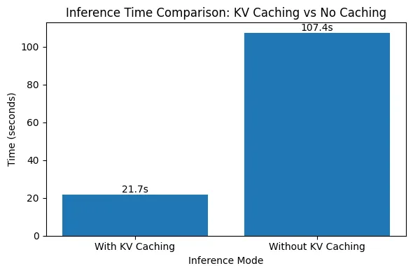
The results clearly demonstrate the impact of KV caching on inference speed. With KV caching enabled, generating 1000 tokens takes around 21.7 seconds, whereas disabling KV caching increases the generation time to over 107 seconds—nearly a 5× slowdown. This sharp difference occurs because, without KV caching, the model recomputes attention over all previously generated tokens at every step, leading to quadratic growth in computation. Check out the
With KV caching, past keys and values are reused, eliminating redundant work and keeping generation time nearly linear as the sequence grows. This experiment highlights why KV caching is essential for efficient, real-world deployment of autoregressive language models.
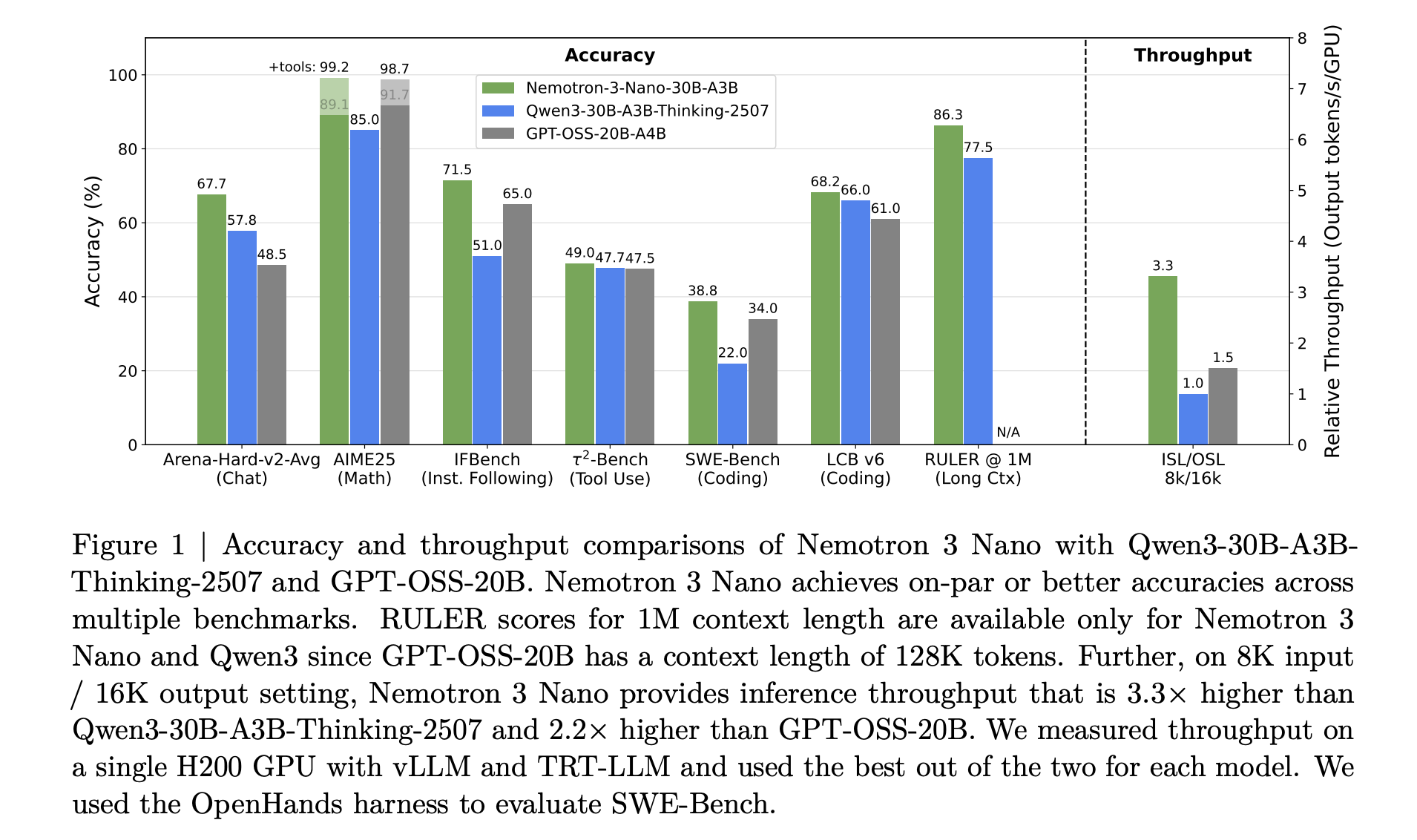
NVIDIA has released the Nemotron 3 family of open models as part of a full stack for agentic AI, including model weights, datasets and reinforcement learning tools. The family has three sizes, Nano, Super and Ultra, and targets multi agent systems that need long context reasoning with tight control over inference cost. Nano has about 30 billion parameters with about 3 billion active per token, Super has about 100 billion parameters with up to 10 billion active per token, and Ultra has about 500 billion parameters with up to 50 billion active per token.
Nemotron 3 is presented as an efficient open model family for agentic applications. The line consists of Nano, Super and Ultra models, each tuned for different workload profiles.
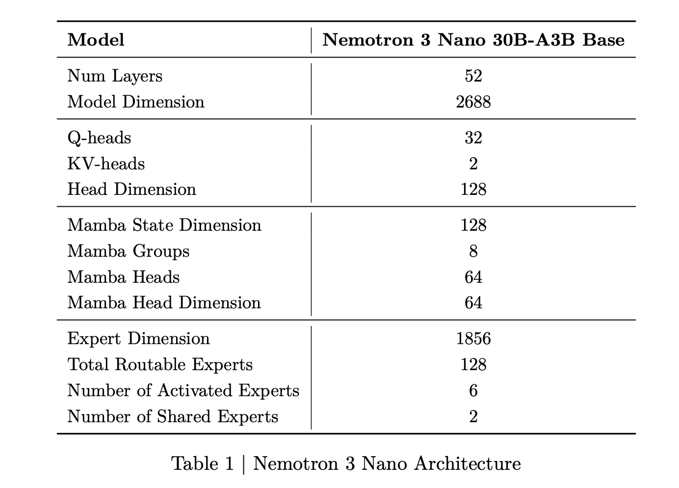
Nemotron 3 Nano is a Mixture of Experts hybrid Mamba Transformer language model with about 31.6 billion parameters. Only about 3.2 billion parameters are active per forward pass, or 3.6 billion including embeddings. This sparse activation allows the model to keep high representational capacity while keeping compute low.
Nemotron 3 Super has about 100 billion parameters with up to 10 billion active per token. Nemotron 3 Ultra scales this design to about 500 billion parameters with up to 50 billion active per token. Super targets high accuracy reasoning for large multi agent applications, while Ultra is intended for complex research and planning workflows.
Nemotron 3 Nano is available now with open weights and recipes, on Hugging Face and as an NVIDIA NIM microservice. Super and Ultra are scheduled for the first half of 2026.
NVIDIA Nemotron 3 Nano delivers about 4 times higher token throughput than Nemotron 2 Nano and reduces reasoning token usage significantly, while supporting a native context length of up to 1 million tokens. This combination is intended for multi agent systems that operate on large workspaces such as long documents and large code bases.
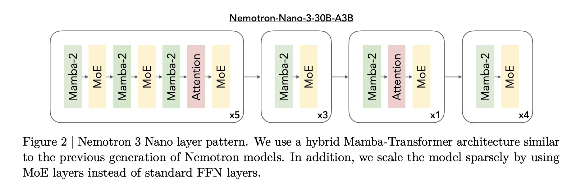
The core design of Nemotron 3 is a Mixture of Experts hybrid Mamba Transformer architecture. The models mix Mamba sequence blocks, attention blocks and sparse expert blocks inside a single stack.
For Nemotron 3 Nano, the research team describes a pattern that interleaves Mamba 2 blocks, attention blocks and MoE blocks. Standard feedforward layers from earlier Nemotron generations are replaced by MoE layers. A learned router selects a small subset of experts per token, for example 6 out of 128 routable experts for Nano, which keeps the active parameter count close to 3.2 billion while the full model holds 31.6 billion parameters.
Mamba 2 handles long range sequence modeling with state space style updates, attention layers provide direct token to token interactions for structure sensitive tasks, and MoE provides parameter scaling without proportional compute scaling. The important point is that most layers are either fast sequence or sparse expert computations, and full attention is used only where it matters most for reasoning.
For Nemotron 3 Super and Ultra, NVIDIA adds LatentMoE. Tokens are projected into a lower dimensional latent space, experts operate in that latent space, then outputs are projected back. This design allows several times more experts at similar communication and compute cost, which supports more specialization across tasks and languages.
Super and Ultra also include multi token prediction. Multiple output heads share a common trunk and predict several future tokens in a single pass. During training this improves optimization, and at inference it enables speculative decoding like execution with fewer full forward passes.
Training data, precision format and context window
Nemotron 3 is trained on large scale text and code data. The research team reports pretraining on about 25 trillion tokens, with more than 3 trillion new unique tokens over the Nemotron 2 generation. Nemotron 3 Nano uses Nemotron Common Crawl v2 point 1, Nemotron CC Code and Nemotron Pretraining Code v2, plus specialized datasets for scientific and reasoning content.
Super and Ultra are trained mostly in NVFP4, a 4 bit floating point format optimized for NVIDIA accelerators. Matrix multiply operations run in NVFP4 while accumulations use higher precision. This reduces memory pressure and improves throughput while keeping accuracy close to standard formats.
All Nemotron 3 models support context windows up to 1 million tokens. The architecture and training pipeline are tuned for long horizon reasoning across this length, which is essential for multi agent environments that pass large traces and shared working memory between agents.
Key Takeaways
Nemotron 3 is a three tier open model family for agentic AI: Nemotron 3 comes in Nano, Super and Ultra variants. Nano has about 30 billion parameters with about 3 billion active per token, Super has about 100 billion parameters with up to 10 billion active per token, and Ultra has about 500 billion parameters with up to 50 billion active per token. The family targets multi agent applications that need efficient long context reasoning.
Hybrid Mamba Transformer MoE with 1 million token context: Nemotron 3 models use a hybrid Mamba 2 plus Transformer architecture with sparse Mixture of Experts and support a 1 million token context window. This design gives long context handling with high throughput, where only a small subset of experts is active per token and attention is used where it is most useful for reasoning.
Latent MoE and multi token prediction in Super and Ultra: The Super and Ultra variants add latent MoE where expert computation happens in a reduced latent space, which lowers communication cost and allows more experts, and multi token prediction heads that generate several future tokens per forward pass. These changes improve quality and enable speculative style speedups for long text and chain of thought workloads.
Large scale training data and NVFP4 precision for efficiency: Nemotron 3 is pretrained on about 25 trillion tokens, with more than 3 trillion new tokens over the previous generation, and Super and Ultra are trained mainly in NVFP4, a 4 bit floating point format for NVIDIA GPUs. This combination improves throughput and reduces memory use while keeping accuracy close to standard precision.
Check out the , and. Feel free to check out our . Also, feel free to follow us on and don’t forget to join our and Subscribe to .

 December 23, 2025
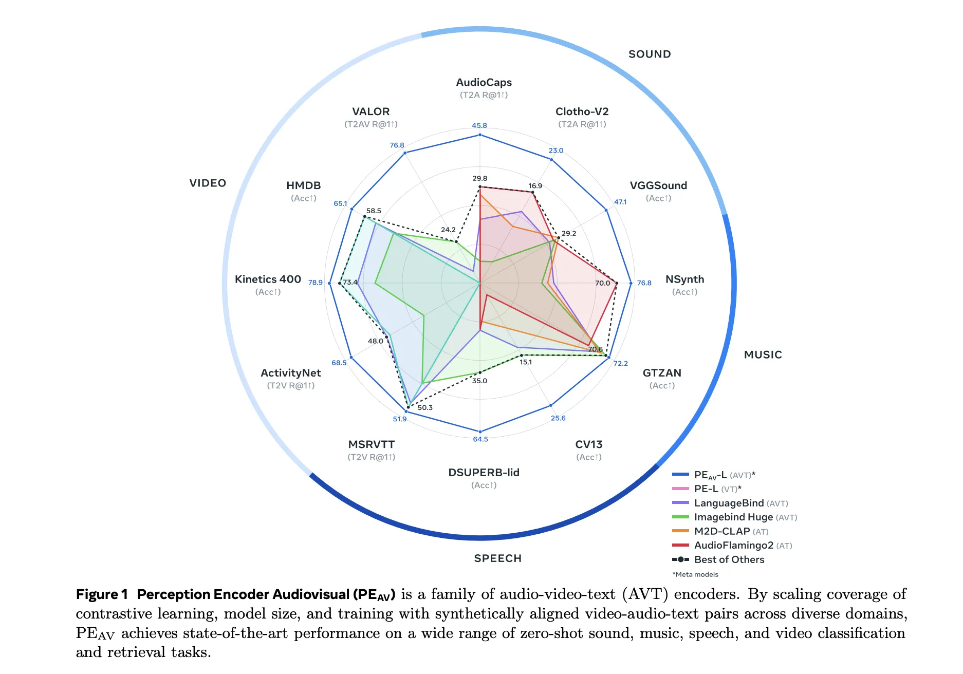


 Installing libraries... (approx 30-60s)")
!pip install smolagents transformers accelerate bitsandbytes ddgs matplotlib pandas -q
import os
import pandas as pd
import matplotlib.pyplot as plt
from smolagents import CodeAgent, Tool, TransformersModel
Installing libraries... (approx 30-60s)")
!pip install smolagents transformers accelerate bitsandbytes ddgs matplotlib pandas -q
import os
import pandas as pd
import matplotlib.pyplot as plt
from smolagents import CodeAgent, Tool, TransformersModel 'fleet_logs.csv' created.")
 Agent is analyzing fleet data... (Check the 'Agent' output below)n")
query = """
1. Load the fleet logs.
2. Find the truck with the worst fuel efficiency (lowest 'fuel_efficiency_kml').
3. For that truck, check if it is overdue for maintenance (threshold is 90 days).
4. Create a bar chart comparing the 'fuel_efficiency_kml' of ALL trucks.
5. Highlight the worst truck in RED and others in GRAY on the chart.
6. Save the chart as 'maintenance_alert.png'.
"""
response = agent.run(query)
print(f"n
Agent is analyzing fleet data... (Check the 'Agent' output below)n")
query = """
1. Load the fleet logs.
2. Find the truck with the worst fuel efficiency (lowest 'fuel_efficiency_kml').
3. For that truck, check if it is overdue for maintenance (threshold is 90 days).
4. Create a bar chart comparing the 'fuel_efficiency_kml' of ALL trucks.
5. Highlight the worst truck in RED and others in GRAY on the chart.
6. Save the chart as 'maintenance_alert.png'.
"""
response = agent.run(query)
print(f"n FINAL REPORT: {response}")
 Displaying Generated Chart:")
img = plt.imread("maintenance_alert.png")
plt.figure(figsize=(10, 5))
plt.imshow(img)
plt.axis('off')
plt.show()
else:
print("
Displaying Generated Chart:")
img = plt.imread("maintenance_alert.png")
plt.figure(figsize=(10, 5))
plt.imshow(img)
plt.axis('off')
plt.show()
else:
print(" No chart image found. Check the agent logs above.")