Just months after releasing M2—a fast, low-cost model designed for agents and code—MiniMax has introduced an enhanced version: MiniMax M2.1.

M2 already stood out for its efficiency, running at roughly 8% of the cost of Claude Sonnet while delivering significantly higher speed. More importantly, it introduced a different computational and reasoning pattern, particularly in how the model structures and executes its thinking during complex code and tool-driven workflows.

M2.1 builds on this foundation, bringing tangible improvements across key areas: better code quality, smarter instruction following, cleaner reasoning, and stronger performance across multiple programming languages. These upgrades extend the original strengths of M2 while staying true to MiniMax’s vision of “Intelligence with Everyone.”

Strengthening the core capabilities of M2, M2.1 is no longer just about better coding—it also produces clearer, more structured outputs across conversations, documentation, and writing.

Core Capabilities and Benchmark Results

• Built for real-world coding and AI-native teams: Designed to support everything from rapid “vibe builds” to complex, production-grade workflows.
• Goes beyond coding: Produces clearer, more structured, and higher-quality outputs across everyday conversations, technical documentation, and writing tasks.
• State-of-the-art multilingual coding performance: Achieves 72.5% on SWE-Multilingual, outperforming Claude Sonnet 4.5 and Gemini 3 Pro across multiple programming languages.
• Strong AppDev & WebDev capabilities: Scores 88.6% on VIBE-Bench, exceeding Claude Sonnet 4.5 and Gemini 3 Pro, with major improvements in native Android, iOS, and modern web development.
• Excellent agent and tool compatibility: Delivers consistent and stable performance across leading coding tools and agent frameworks, including Claude Code, Droid (Factory AI), Cline, Kilo Code, Roo Code, BlackBox, and more.
• Robust context management support: Works reliably with advanced context mechanisms such as Skill.md, Claude.md / agent.md / cursorrule, and Slash Commands, enabling scalable agent workflows.
• Automatic caching, zero configuration: Built-in caching works out of the box to reduce latency, lower costs, and deliver a smoother overall experience.

Getting Started with MiniMax M2.1

To get started with MiniMax M2.1, you’ll need an API key from the . You can generate one from the MiniMax user console.

Once issued, store the API key securely and avoid exposing it in code repositories or public environments.

Installing & Setting up the dependencies

MiniMax supports both the Anthropic and OpenAI API formats, making it easy to integrate MiniMax models into existing workflows with minimal configuration changes—whether you’re using Anthropic-style message APIs or OpenAI-compatible setups.

pip install anthropic

import os
from getpass import getpass
os.environ['ANTHROPIC_BASE_URL'] = 'https://api.minimax.io/anthropic'
os.environ['ANTHROPIC_API_KEY'] = getpass('Enter MiniMax API Key: ')

With just this minimal setup, you’re ready to start using the model.

Sending Requests to the Model

MiniMax M2.1 returns structured outputs that separate internal reasoning (thinking) from the final response (text). This allows you to observe how the model interprets intent and plans its answer before producing the user-facing output.

import anthropic

client = anthropic.Anthropic()

message = client.messages.create(
    model="MiniMax-M2.1",
    max_tokens=1000,
    system="You are a helpful assistant.",
    messages=[
        {
            "role": "user",
            "content": [
                {
                    "type": "text",
                    "text": "Hi, how are you?"
                }
            ]
        }
    ]
)

for block in message.content:
    if block.type == "thinking":
        print(f"Thinking:n{block.thinking}n")
    elif block.type == "text":
        print(f"Text:n{block.text}n")

Thinking:
The user is just asking how I am doing. This is a friendly greeting, so I should respond in a warm, conversational way. I'll keep it simple and friendly.

Text:
Hi! I'm doing well, thanks for asking! 

I'm ready to help you with whatever you need today. Whether it's coding, answering questions, brainstorming ideas, or just chatting, I'm here for you.

What can I help you with?

What makes MiniMax stand out is the visibility into its reasoning process. Before producing the final response, the model explicitly reasons about the user’s intent, tone, and expected style—ensuring the answer is appropriate and context-aware. 

By cleanly separating reasoning from responses, the model becomes easier to interpret, debug, and trust, especially in complex agent-based or multi-step workflows, and with M2.1 this clarity is paired with faster responses, more concise reasoning, and substantially reduced token consumption compared to M2.

Testing the Model’s Coding Capabilities

MiniMax M2 stands out for its native mastery of Interleaved Thinking, allowing it to dynamically plan and adapt within complex coding and tool-based workflows, and M2.1 extends this capability with improved code quality, more precise instruction following, clearer reasoning, and stronger performance across programming languages—particularly in handling composite instruction constraints as seen in OctoCodingBench—making it ready for office automation.

To evaluate these capabilities in practice, let’s test the model using a structured coding prompt that includes multiple constraints and real-world engineering requirements.

import anthropic

client = anthropic.Anthropic()

def run_test(prompt: str, title: str):
    print(f"n{'='*80}")
    print(f"TEST: {title}")
    print(f"{'='*80}n")

    message = client.messages.create(
        model="MiniMax-M2.1",
        max_tokens=10000,
        system=(
            "You are a senior software engineer. "
            "Write production-quality code with clear structure, "
            "explicit assumptions, and minimal but sufficient reasoning. "
            "Avoid unnecessary verbosity."
        ),
        messages=[
            {
                "role": "user",
                "content": [{"type": "text", "text": prompt}]
            }
        ]
    )

    for block in message.content:
        if block.type == "thinking":
            print(" Thinking:n", block.thinking, "n")
        elif block.type == "text":
            print(" Output:n", block.text, "n")

PROMPT= """
Design a small Python service that processes user events.

Requirements:
1. Events arrive as dictionaries with keys: user_id, event_type, timestamp.
2. Validate input strictly (types + required keys).
3. Aggregate events per user in memory.
4. Expose two functions:
   - ingest_event(event: dict) -> None
   - get_user_summary(user_id: str) -> dict
5. Code must be:
   - Testable
   - Thread-safe
   - Easily extensible for new event types
6. Do NOT use external libraries.

Provide:
- Code only
- Brief inline comments where needed
"""

run_test(prompt=PROMPT, title="Instruction Following + Architecture")

This test uses a deliberately structured and constraint-heavy prompt designed to evaluate more than just code generation. The prompt requires strict input validation, in-memory state management, thread safety, testability, and extensibility—all without relying on external libraries.

By combining architectural decisions with multiple non-trivial constraints, the prompt operates at a medium-to-high complexity level, making it well-suited for assessing how effectively MiniMax M2.1 follows instructions, reasons through design trade-offs, and produces production-quality code rather than isolated snippets.

Model Reasoning & Output

The model reasons through key architectural trade-offs before coding, carefully balancing flexibility, memory usage, and extensibility. It evaluates multiple approaches to event aggregation and deliberately chooses raw event storage to enable future extensions without modifying ingestion logic. 

Thread safety is explicitly handled through locking, and strict input validation is planned to ensure data correctness, reflecting a real-world, engineering-first mindset rather than jumping straight to implementation.

This thoughtful reasoning is reflected in the final output, which demonstrates strong code quality through clear structure, meaningful naming, type hints, and a thread-safe design aligned with production standards. The solution follows all prompt constraints accurately—covering validation, in-memory aggregation, extensibility, and the absence of external dependencies—while maintaining clean, focused logic that avoids unnecessary complexity and remains easy to maintain.

import threading
from typing import Dict, List, Any

class EventProcessor:
    """
    Thread-safe event processor that aggregates user events in memory.
    Validates input strictly and supports easy extension for new event types.
    """
    
    def __init__(self) -> None:
        # Stores events per user: user_id -> list of event dictionaries
        self._user_events: Dict[str, List[Dict[str, Any]]] = {}
        # Lock for thread-safe access
        self._lock = threading.Lock()
    
    def ingest_event(self, event: dict) -> None:
        """
        Validate and ingest a single event.
        Strictly validates types and presence of required keys.
        """
        # Validate event is a dictionary
        if not isinstance(event, dict):
            raise ValueError("Event must be a dictionary")
        
        # Validate required keys and their types
        required_keys = {
            'user_id': str,
            'event_type': str,
            'timestamp': (str, int, float)  # Accept string or numeric timestamp
        }
        
        for key, expected_type in required_keys.items():
            if key not in event:
                raise ValueError(f"Missing required key: '{key}'")
            if not isinstance(event[key], expected_type):
                raise ValueError(f"Key '{key}' must be of type {expected_type.__name__}")
        
        # Thread-safe event storage
        with self._lock:
            user_id = event['user_id']
            if user_id not in self._user_events:
                self._user_events[user_id] = []
            self._user_events[user_id].append(event)
    
    def get_user_summary(self, user_id: str) -> dict:
        """
        Generate summary for a specific user.
        Returns aggregated event counts and timestamps.
        """
        if not isinstance(user_id, str):
            raise ValueError("user_id must be a string")
        
        with self._lock:
            user_events = self._user_events.get(user_id, [])
            
            # Aggregate event counts
            event_counts = {}
            timestamps = []
            
            for event in user_events:
                event_type = event['event_type']
                event_counts[event_type] = event_counts.get(event_type, 0) + 1
                timestamps.append(event['timestamp'])
            
            return {
                'user_id': user_id,
                'total_events': len(user_events),
                'event_counts': event_counts,
                'timestamps': sorted(timestamps) if timestamps else []
            }
```

**Key Design Choices:**

1. **Thread Safety**: Uses `threading.Lock` to protect shared state during concurrent access
2. **Input Validation**: Strict type checking for required keys with clear error messages
3. **Extensibility**: 
   - New event types automatically handled by dynamic counting
   - Easy to add new aggregations in `get_user_summary`
4. **Testability**: Clear separation of concerns, easy to mock for unit tests
5. **Memory Efficiency**: Stores only essential data (event dictionaries)

**Usage Example:**
```python
processor = EventProcessor()

# Ingest events
processor.ingest_event({
    'user_id': 'user123',
    'event_type': 'login',
    'timestamp': '2023-01-01T10:00:00Z'
})

# Get user summary
summary = processor.get_user_summary('user123')
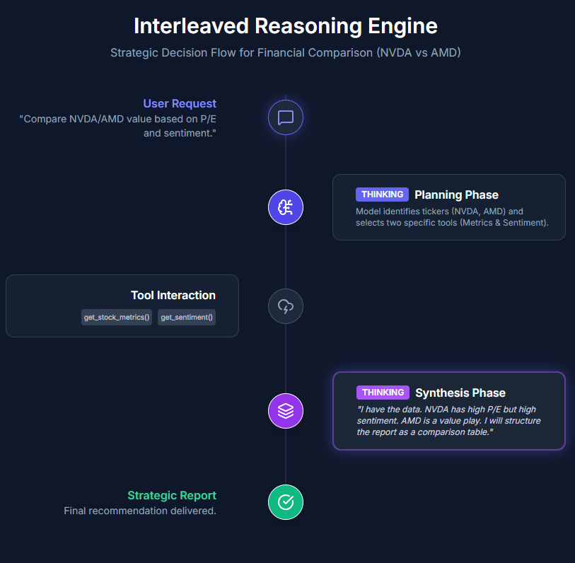
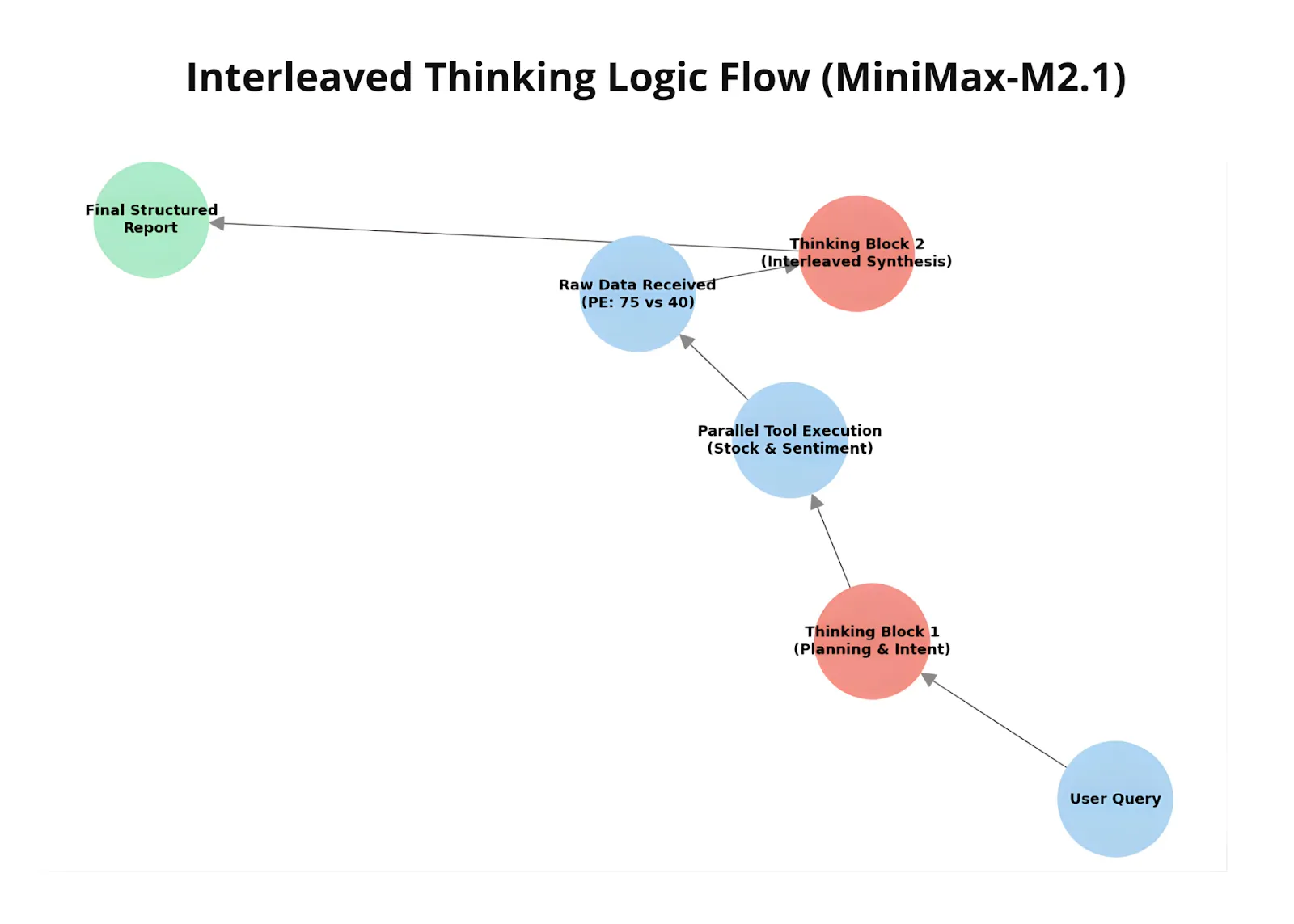
print(summary)

Model’s Interleaved Thinking in Action

Let’s now see MiniMax M2.1’s interleaved thinking in action. We ask the model to compare two organizations based on P/E ratio and sentiment, using two dummy tools to clearly observe how the workflow operates. 

This example demonstrates how M2.1 interacts with external tools in a controlled, agent-style setup. One tool simulates fetching stock metrics, while the other provides sentiment analysis, with both returning locally generated responses. As the model receives these tool outputs, it incorporates them into its reasoning and adjusts its final comparison accordingly.

Defining the tools

import anthropic
import json

client = anthropic.Anthropic()

def get_stock_metrics(ticker):
    data = {
        "NVDA": {"price": 130, "pe": 75.2},
        "AMD": {"price": 150, "pe": 40.5}
    }
    return json.dumps(data.get(ticker, "Ticker not found"))

def get_sentiment_analysis(company_name):
    sentiments = {"NVIDIA": 0.85, "AMD": 0.42}
    return f"Sentiment score for {company_name}: {sentiments.get(company_name, 0.0)}"

tools = [
    {
        "name": "get_stock_metrics",
        "description": "Get price and P/E ratio.",
        "input_schema": {
            "type": "object",
            "properties": {"ticker": {"type": "string"}},
            "required": ["ticker"]
        }
    },
    {
        "name": "get_sentiment_analysis",
        "description": "Get news sentiment score.",
        "input_schema": {
            "type": "object",
            "properties": {"company_name": {"type": "string"}},
            "required": ["company_name"]
        }
    }
]

Model Execution with Tool Interaction

messages = [{"role": "user", "content": "Compare NVDA and AMD value based on P/E and sentiment."}]
running = True

print(f" [USER]: {messages[0]['content']}")

while running:
    # Get model response
    response = client.messages.create(
        model="MiniMax-M2.1",
        max_tokens=4096,
        messages=messages,
        tools=tools,
    )

    messages.append({"role": "assistant", "content": response.content})

    tool_results = []
    has_tool_use = False

    for block in response.content:
        if block.type == "thinking":
            print(f"n [THINKING]:n{block.thinking}")
        
        elif block.type == "text":
            print(f"n [MODEL]: {block.text}")
            if not any(b.type == "tool_use" for b in response.content):
                running = False
        
        elif block.type == "tool_use":
            has_tool_use = True
            print(f" [TOOL CALL]: {block.name}({block.input})")
            
            # Execute the correct mock function
            if block.name == "get_stock_metrics":
                result = get_stock_metrics(block.input['ticker'])
            elif block.name == "get_sentiment_analysis":
                result = get_sentiment_analysis(block.input['company_name'])
            
            # Add to the results list for this turn
            tool_results.append({
                "type": "tool_result",
                "tool_use_id": block.id,
                "content": result
            })

    if has_tool_use:
        messages.append({"role": "user", "content": tool_results})
    else:
        running = False

print("n Conversation Complete.")

During execution, the model decides when and which tool to call, receives the corresponding tool results, and then updates its reasoning and final response based on that data. This showcases M2.1’s ability to interleave reasoning, tool usage, and response generation—adapting its output dynamically as new information becomes available.

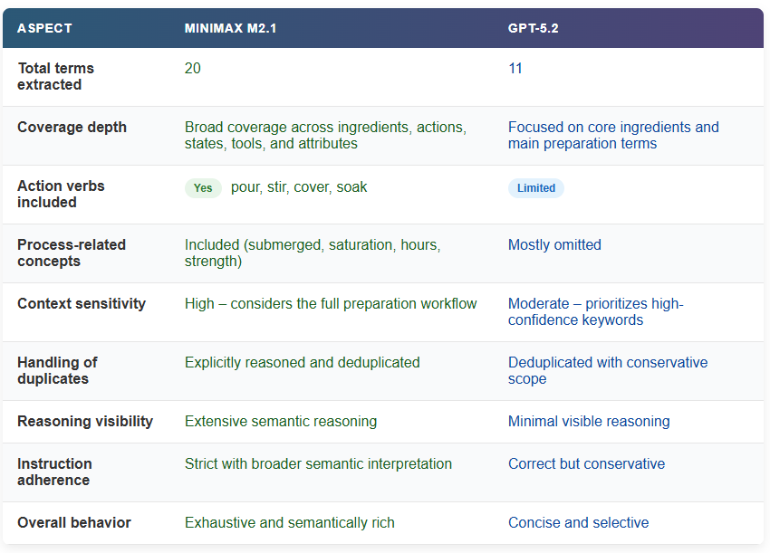
Comparison with OpenAI’s GPT-5.2

Finally, we compare MiniMax M2.1 with GPT-5.2 using a compact multilingual instruction-following prompt. The task requires the model to identify coffee-related terms from a Spanish passage, translate only those terms into English, remove duplicates, and return the result in a strictly formatted numbered list.

To run this code block, you’ll need an OpenAI API key, which can be generated from the .

import os
from getpass import getpass
os.environ['OPENAI_API_KEY'] = getpass ('Enter OpenAI API Key: ')

input_text = """
¡Preparar café Cold Brew es un proceso sencillo y refrescante!
Todo lo que necesitas son granos de café molido grueso y agua fría.
Comienza añadiendo el café molido a un recipiente o jarra grande.
Luego, vierte agua fría, asegurándote de que todos los granos de café
estén completamente sumergidos.
Remueve la mezcla suavemente para garantizar una saturación uniforme.
Cubre el recipiente y déjalo en remojo en el refrigerador durante al
menos 12 a 24 horas, dependiendo de la fuerza deseada.
"""

prompt = f"""
The following text is written in Spanish.

Task:
1. Identify all words in the text that are related to coffee or coffee preparation.
2. Translate ONLY those words into English.
3. Remove duplicates (each word should appear only once).
4. Present the result as a numbered list.

Rules:
- Do NOT include explanations.
- Do NOT include non-coffee-related words.
- Do NOT include Spanish words in the final output.

Text:
<{input_text}>
"""

from openai import OpenAI
client = OpenAI()

response = client.responses.create(
    model="gpt-5.2",
    input=prompt
)

print(response.output_text)

import anthropic

client = anthropic.Anthropic()

message = client.messages.create(
    model="MiniMax-M2.1",
    max_tokens=10000,
    system="You are a helpful assistant.",
    messages=[
        {
            "role": "user",
            "content": [
                {
                    "type": "text",
                    "text": prompt
                }
            ]
        }
    ]
)

for block in message.content:
    if block.type == "thinking":
        print(f"Thinking:n{block.thinking}n")
    elif block.type == "text":
        print(f"Text:n{block.text}n")

When comparing the outputs, MiniMax M2.1 produces a noticeably broader and more granular set of coffee-related terms than GPT-5.2. M2.1 identifies not only core nouns like coffee, beans, and water, but also preparation actions (pour, stir, cover), process-related states (submerged, soak), and contextual attributes (cold, coarse, strength, hours). 

This indicates a deeper semantic pass over the text, where the model reasons through the entire preparation workflow rather than extracting only the most obvious keywords.

This difference is also reflected in the reasoning process. M2.1 explicitly analyzes context, resolves edge cases (such as borrowed English terms like Cold Brew), considers duplicates, and deliberates on whether certain adjectives or verbs qualify as coffee-related before finalizing the list. GPT-5.2, by contrast, delivers a shorter and more conservative output focused on high-confidence terms, with less visible reasoning depth. 

Together, this highlights M2.1’s stronger instruction adherence and semantic coverage, especially for tasks that require careful filtering, translation, and strict output control.

The post appeared first on .

In this tutorial, we build an advanced, fully autonomous logistics simulation in which multiple smart delivery trucks operate within a dynamic city-wide road network. We design the system so that each truck behaves as an agent capable of bidding on delivery orders, planning optimal routes, managing battery levels, seeking charging stations, and maximizing profit through self-interested decision-making. Through each code snippet, we explore how agentic behaviors emerge from simple rules, how competition shapes order allocation, and how a graph-based world enables realistic movement, routing, and resource constraints. Check out the .

import networkx as nx
import matplotlib.pyplot as plt
import random
import time
from IPython.display import clear_output
from dataclasses import dataclass, field
from typing import List, Dict, Optional


NUM_NODES = 30
CONNECTION_RADIUS = 0.25
NUM_AGENTS = 5
STARTING_BALANCE = 1000
FUEL_PRICE = 2.0
PAYOUT_MULTIPLIER = 5.0
BATTERY_CAPACITY = 100
CRITICAL_BATTERY = 25


@dataclass
class Order:
   id: str
   target_node: int
   weight_kg: int
   payout: float
   status: str = "pending"


class AgenticTruck:
   def __init__(self, agent_id, start_node, graph, capacity=100):
       self.id = agent_id
       self.current_node = start_node
       self.graph = graph
       self.battery = BATTERY_CAPACITY
       self.balance = STARTING_BALANCE
       self.capacity = capacity
       self.state = "IDLE"
       self.path: List[int] = []
       self.current_order: Optional[Order] = None
       self.target_node: int = start_node

We set up all the core building blocks of the simulation, including imports, global parameters, and the basic data structures. We also define the AgenticTruck class and initialize key attributes, including position, battery, balance, and operating state. We lay the foundation for all agent behaviors to evolve. Check out the .

 def get_path_cost(self, start, end):
       try:
           length = nx.shortest_path_length(self.graph, start, end, weight='weight')
           path = nx.shortest_path(self.graph, start, end, weight='weight')
           return length, path
       except nx.NetworkXNoPath:
           return float('inf'), []


   def find_nearest_charger(self):
       chargers = [n for n, attr in self.graph.nodes(data=True) if attr.get('type') == 'charger']
       best_charger = None
       min_dist = float('inf')
       best_path = []
       for charger in chargers:
           dist, path = self.get_path_cost(self.current_node, charger)
           if dist < min_dist:
               min_dist = dist
               best_charger = charger
               best_path = path
       return best_charger, best_path


   def calculate_bid(self, order):
       if order.weight_kg > self.capacity:
           return float('inf')
       if self.state != "IDLE" or self.battery < CRITICAL_BATTERY:
           return float('inf')
       dist_to_target, _ = self.get_path_cost(self.current_node, order.target_node)
       fuel_cost = dist_to_target * FUEL_PRICE
       expected_profit = order.payout - fuel_cost
       if expected_profit < 10:
           return float('inf')
       return dist_to_target


   def assign_order(self, order):
       self.current_order = order
       self.state = "MOVING"
       self.target_node = order.target_node
       _, self.path = self.get_path_cost(self.current_node, self.target_node)
       if self.path: self.path.pop(0)


   def go_charge(self):
       charger_node, path = self.find_nearest_charger()
       if charger_node is not None:
           self.state = "TO_CHARGER"
           self.target_node = charger_node
           self.path = path
           if self.path: self.path.pop(0)

We implement advanced decision-making logic for the trucks. We calculate shortest paths, identify nearby charging stations, and evaluate whether an order is profitable and feasible. We also prepare the truck to accept assignments or proactively seek charging when needed. Check out the .

 def step(self):
       if self.state == "IDLE" and self.battery < CRITICAL_BATTERY:
           self.go_charge()


       if self.state == "CHARGING":
           self.battery += 10
           self.balance -= 5
           if self.battery >= 100:
               self.battery = 100
               self.state = "IDLE"
           return


       if self.path:
           next_node = self.path[0]
           edge_data = self.graph.get_edge_data(self.current_node, next_node)
           distance = edge_data['weight']
           self.current_node = next_node
           self.path.pop(0)
           self.battery -= (distance * 2)
           self.balance -= (distance * FUEL_PRICE)


           if not self.path:
               if self.state == "MOVING":
                   self.balance += self.current_order.payout
                   self.current_order.status = "completed"
                   self.current_order = None
                   self.state = "IDLE"
               elif self.state == "TO_CHARGER":
                   self.state = "CHARGING"

We manage the step-by-step actions of each truck as the simulation runs. We handle battery recharging, financial impacts of movement, fuel consumption, and order completion. We ensure that agents transition smoothly between states, such as moving, charging, and idling. Check out the .

class Simulation:
   def __init__(self):
       self.setup_graph()
       self.setup_agents()
       self.orders = []
       self.order_count = 0


   def setup_graph(self):
       self.G = nx.random_geometric_graph(NUM_NODES, CONNECTION_RADIUS)
       for (u, v) in self.G.edges():
           self.G.edges[u, v]['weight'] = random.uniform(1.0, 3.0)
       for i in self.G.nodes():
           r = random.random()
           if r < 0.15:
               self.G.nodes[i]['type'] = 'charger'
               self.G.nodes[i]['color'] = 'red'
           else:
               self.G.nodes[i]['type'] = 'house'
               self.G.nodes[i]['color'] = '#A0CBE2'


   def setup_agents(self):
       self.agents = []
       for i in range(NUM_AGENTS):
           start_node = random.randint(0, NUM_NODES-1)
           cap = random.choice([50, 100, 200])
           self.agents.append(AgenticTruck(i, start_node, self.G, capacity=cap))


   def generate_order(self):
       target = random.randint(0, NUM_NODES-1)
       weight = random.randint(10, 120)
       payout = random.randint(50, 200)
       order = Order(id=f"ORD-{self.order_count}", target_node=target, weight_kg=weight, payout=payout)
       self.orders.append(order)
       self.order_count += 1
       return order


   def run_market(self):
       for order in self.orders:
           if order.status == "pending":
               bids = {agent: agent.calculate_bid(order) for agent in self.agents}
               valid_bids = {k: v for k, v in bids.items() if v != float('inf')}
               if valid_bids:
                   winner = min(valid_bids, key=valid_bids.get)
                   winner.assign_order(order)
                   order.status = "assigned"

We create the simulated world and orchestrate agent interactions. We generate the graph-based city, spawn trucks with varying capacities, and produce new delivery orders. We also implement a simple market where agents bid for tasks based on profitability and distance. Check out the .

  def step(self):
       if random.random() < 0.3:
           self.generate_order()
       self.run_market()
       for agent in self.agents:
           agent.step()


   def visualize(self, step_num):
       clear_output(wait=True)
       plt.figure(figsize=(10, 8))
       pos = nx.get_node_attributes(self.G, 'pos')
       node_colors = [self.G.nodes[n]['color'] for n in self.G.nodes()]
       nx.draw(self.G, pos, node_color=node_colors, with_labels=True, node_size=300, edge_color='gray', alpha=0.6)


       for agent in self.agents:
           x, y = pos[agent.current_node]
           jitter_x = x + random.uniform(-0.02, 0.02)
           jitter_y = y + random.uniform(-0.02, 0.02)
           color = 'green' if agent.state == "IDLE" else ('orange' if agent.state == "MOVING" else 'red')
           plt.plot(jitter_x, jitter_y, marker='s', markersize=12, color=color, markeredgecolor='black')
           plt.text(jitter_x, jitter_y+0.03, f"A{agent.id}n${int(agent.balance)}n{int(agent.battery)}%",
                    fontsize=8, ha='center', fontweight='bold', bbox=dict(facecolor='white', alpha=0.7, pad=1))


       for order in self.orders:
           if order.status in ["assigned", "pending"]:
               ox, oy = pos[order.target_node]
               plt.plot(ox, oy, marker='*', markersize=15, color='gold', markeredgecolor='black')


       plt.title(f"Graph-Based Logistics Swarm | Step: {step_num}nRed Nodes = Chargers | Gold Stars = Orders", fontsize=14)
       plt.show()




print("Initializing Advanced Simulation...")
sim = Simulation()


for t in range(60):
   sim.step()
   sim.visualize(t)
   time.sleep(0.5)


print("Simulation Finished.")

We step through the full simulation loop and visualize the logistics swarm in real time. We update agent states, draw the network, display active orders, and animate each truck’s movement. By running this loop, we observe the emergent coordination and competition that define our multi-agent logistics ecosystem.

In conclusion, we saw how the individual components, graph generation, autonomous routing, battery management, auctions, and visualization, come together to form a living, evolving system of agentic trucks. We watch as agents negotiate workloads, compete for profitable opportunities, and respond to environmental pressures such as distance, fuel costs, and charging needs. By running the simulation, we observe emergent dynamics that mirror real-world fleet behavior, providing a powerful sandbox for experimenting with logistics intelligence.

Check out the . Also, feel free to follow us on  and don’t forget to join our  and Subscribe to . Wait! are you on telegram? 

The post appeared first on .

Agentic AI systems sit on top of large language models and connect to tools, memory, and external environments. They already support scientific discovery, software development, and clinical research, yet they still struggle with unreliable tool use, weak long horizon planning, and poor generalization. The latest research paper ‘Adaptation of Agentic AI‘ from Stanford, Harvard, UC Berkeley, Caltech proposes a unified view of how these systems should adapt and maps existing methods into a compact, mathematically defined framework.

How this research paper models an agentic AI system?

The research survey models an agentic AI system as a foundation model agent along with 3 key components. A planning module decomposes goals into sequences of actions, using static procedures such as Chain-of-Thought and Tree-of-Thought, or dynamic procedures such as ReAct and Reflexion that react to feedback. A tool use module connects the agent to web search engines, APIs, code execution environments, Model Context Protocols, and browser automation. A memory module stores short term context and long term knowledge, accessed through retrieval augmented generation. Adaptation changes prompts or parameters for these components using supervised fine tuning, preference based methods such as Direct Preference Optimization, reinforcement learning methods such as Proximal Policy Optimization and Group Relative Policy Optimization, and parameter efficient techniques such as low rank adaptation.

Four adaptation paradigms

The framework defines 4 adaptation paradigms by combining 2 binary choices. The first dimension is the target, agent adaptation versus tool adaptation. The second dimension is the supervision signal, tool execution versus agent output. This yields A1 and A2 for adapting the agent, and T1 and T2 for adapting tools.

A1, Tool Execution Signaled Agent Adaptation, optimizes the agent using feedback derived from tool execution. A2, Agent Output Signaled Agent Adaptation, optimizes the agent using a signal defined only on its final outputs. T1, Agent-Agnostic Tool Adaptation, optimizes tools without referring to a particular agent. T2, Agent-Supervised Tool Adaptation, optimizes tools under supervision from a fixed agent.

A1, learning from verifiable tool feedback

In A1, the agent receives an input x, produces a structured tool call a, the tools return a result y, and the learning objective O_tool measures tool success, for example execution correctness or retrieval quality. The paper covers both supervised imitation of successful tool trajectories and reinforcement learning that uses verifiable tool outcomes as reward.

Toolformer, ToolAlpaca, and Gorilla illustrate supervised A1 methods, since each uses execution results of real tools to construct or filter training traces before imitation. All of them keep the supervision signal defined at the tool behavior level, not at the final answer level.

DeepRetrieval is a central A1 reinforcement learning example. It frames query reformulation as a Markov decision process where the state is the user query, the action is a rewritten query, and the reward combines retrieval metrics such as Recall and nDCG, a format term, and, for text to SQL, SQL execution accuracy. The policy is trained with KL regularized Proximal Policy Optimization and the same objective covers literature search, corpus question answering, and text to SQL.

A2, learning from final agent outputs

A2 covers cases where the optimization objective O_agent depends only on the final output o produced by the agent, even when the agent uses tools internally. The survey shows that supervising only o is not enough to teach tools, because the agent can ignore tools and still improve likelihood. Effective A2 systems therefore combine supervision on tool calls with supervision on final answers, or assign sparse rewards such as exact match accuracy to o and propagate them back through the full trajectory.

T1, agent agnostic tool training

T1 freezes the main agent and optimizes tools so that they are broadly reusable. The objective O_tool depends only on tool outputs and is measured by metrics such as retrieval accuracy, ranking quality, simulation fidelity, or downstream task success. A1 trained search policies, such as DeepRetrieval, can later be reused as T1 tools inside new agentic systems without modifying the main agent.

T2, tools optimized under a frozen agent

T2 assumes a powerful but fixed agent A, which is common when the agent is a closed source foundation model. The tool executes calls and returns results that the agent then uses to produce o. The optimization objective again lives on O_agent, but the trainable parameters belong to the tool. The paper describes quality weighted training, target based training, and reinforcement learning variants that all derive learning signals for the tool from the final agent outputs.

The survey treats long term memory as a special case of T2. Memory is an external store written and read through learned functions, and the agent remains frozen. Recent T2 systems include s3, which trains a 7 billion parameter searcher that maximizes a Gain Beyond RAG reward defined by a frozen generator, and AgentFlow, which trains a planner to orchestrate mostly frozen Qwen2.5 based modules using Flow GRPO.

Key Takeaways

• The research defines a precise 4 paradigm framework for adapting agentic AI by crossing 2 dimensions, whether adaptation targets the agent or tools, and whether the supervision signal comes from tool execution or from final agent outputs.
• A1 methods such as Toolformer, ToolAlpaca, Gorilla, and DeepRetrieval adapt the agent directly from verifiable tool feedback, including retrieval metrics, SQL execution accuracy, and code execution results, often optimized with KL regularized Proximal Policy Optimization.
• A2 methods optimize the agent from signals on final outputs, for example answer accuracy, and the paper shows that systems must still supervise tool calls or propagate sparse rewards through full trajectories, otherwise the agent can ignore tools while still improving likelihood.
• T1 and T2 shift learning to tools and memory, T1 trains generally useful retrievers, searchers, and simulators without a specific agent in mind, while T2 adapts tools under a frozen agent, as in s3 and AgentFlow where a fixed generator supervises a learned searcher and planner.
• The research team introduce an adaptation landscape that relates monolithic versus modular and local versus systemic control, and they argue that practical systems will combine rare A1 or A2 updates on a strong base model with frequent T1 and T2 adaptation of retrievers, search policies, simulators, and memory for robustness and scalability.

Check out the  and . Also, feel free to follow us on  and don’t forget to join our  and Subscribe to . Wait! are you on telegram? 

The post appeared first on .

Genomic prediction and design now require models that connect local motifs with megabase scale regulatory context and that operate across many organisms. Nucleotide Transformer v3, or NTv3, is InstaDeep’s new multi species genomics foundation model for this setting. It unifies representation learning, functional track and genome annotation prediction, and controllable sequence generation in a single backbone that runs on 1 Mb contexts at single nucleotide resolution.

Earlier Nucleotide Transformer models already showed that self supervised pretraining on thousands of genomes yields strong features for molecular phenotype prediction. The original series included models from 50M to 2.5B parameters trained on 3,200 human genomes and 850 additional genomes from diverse species. NTv3 keeps this sequence only pretraining idea but extends it to longer contexts and adds explicit functional supervision and a generative mode.

Architecture for 1 Mb genomic windows

NTv3 uses a U-Net style architecture that targets very long genomic windows. A convolutional downsampling tower compresses the input sequence, a transformer stack models long range dependencies in that compressed space, and a deconvolution tower restores base level resolution for prediction and generation. Inputs are tokenized at the character level over A, T, C, G, N with special tokens such as <unk>, <pad>, <mask>, <cls>, <eos>, and <bos>. Sequence length must be a multiple of 128 tokens, and the reference implementation uses padding to enforce this constraint. All public checkpoints use single base tokenization with a vocabulary size of 11 tokens.

The smallest public model, NTv3 8M pre, has about 7.69M parameters with hidden dimension 256, FFN dimension 1,024, 2 transformer layers, 8 attention heads, and 7 downsample stages. At the high end, NTv3 650M uses hidden dimension 1,536, FFN dimension 6,144, 12 transformer layers, 24 attention heads, and 7 downsample stages, and adds conditioning layers for species specific prediction heads.

Training data

The NTv3 model is pretrained on 9 trillion base pairs from the OpenGenome2 resource using base resolution masked language modeling. After this stage, the model is post trained with a joint objective that integrates continued self supervision with supervised learning on approximately 16,000 functional tracks and annotation labels from 24 animal and plant species.

Performance and Ntv3 Benchmark

After post training NTv3 achieves state of the art accuracy for functional track prediction and genome annotation across species. It outperforms strong sequence to function models and previous genomic foundation models on existing public benchmarks and on the new Ntv3 Benchmark, which is defined as a controlled downstream fine tuning suite with standardized 32 kb input windows and base resolution outputs.

The Ntv3 Benchmark currently consists of 106 long range, single nucleotide, cross assay, cross species tasks. Because NTv3 sees thousands of tracks across 24 species during post training, the model learns a shared regulatory grammar that transfers between organisms and assays and supports coherent long range genome to function inference.

From prediction to controllable sequence generation

Beyond prediction, NTv3 can be fine tuned into a controllable generative model via masked diffusion language modeling. In this mode the model receives conditioning signals that encode desired enhancer activity levels and promoter selectivity, and it fills masked spans in the DNA sequence in a way that is consistent with those conditions.

In experiments described in the launch materials, the team designs 1,000 enhancer sequences with specified activity and promoter specificity and validates them in vitro using STARR seq assays in collaboration with the Stark Lab. The results show that these generated enhancers recover the intended ordering of activity levels and reach more than 2 times improved promoter specificity compared with baselines.

Key Takeaways

1. NTv3 is a long range, multi species genomics foundation model: It unifies representation learning, functional track prediction, genome annotation, and controllable sequence generation in a single U Net style architecture that supports 1 Mb nucleotide resolution context across 24 animal and plant species.
2. The model is trained on 9 trillion base pairs with joint self supervised and supervised objectives: NTv3 is pretrained on 9 trillion base pairs from OpenGenome2 with base resolution masked language modeling, then post trained on more than 16,000 functional tracks and annotation labels from 24 species using a joint objective that mixes continued self supervision with supervised learning.
3. NTv3 achieves state of the art performance on the Ntv3 Benchmark: After post training, NTv3 reaches state of the art accuracy for functional track prediction and genome annotation across species and outperforms previous sequence to function models and genomics foundation models on public benchmarks and on the Ntv3 Benchmark, which contains 106 standardized long range downstream tasks with 32 kb input and base resolution outputs.
4. The same backbone supports controllable enhancer design validated with STARR seq: NTv3 can be fine tuned as a controllable generative model using masked diffusion language modeling to design enhancer sequences with specified activity levels and promoter selectivity, and these designs are validated experimentally with STARR seq assays that confirm the intended activity ordering and improved promoter specificity.

Check out the ,  and . Also, feel free to follow us on  and don’t forget to join our  and Subscribe to . Wait! are you on telegram? 

The post appeared first on .

Google Health AI team has released MedASR, an open weights medical speech to text model that targets clinical dictation and physician patient conversations and is designed to plug directly into modern AI workflows.

What MedASR is and where it fits?

MedASR is a speech to text model based on the Conformer architecture and is pre trained for medical dictation and transcription. It is positioned as a starting point for developers who want to build healthcare based voice applications such as radiology dictation tools or visit note capture systems.

The model has 105 million parameters and accepts mono channel audio at 16000 hertz with 16 bit integer waveforms. It produces text only output, so it drops directly into downstream natural language processing or generative models such as MedGemma.

MedASR sits inside the Health AI Developer Foundations portfolio, alongside MedGemma, MedSigLIP and other domain specific medical models that share common terms of use and a consistent governance story.

Training data and domain specialization

MedASR is trained on a diverse corpus of de identified medical speech. The dataset includes about 5000 hours of physician dictations and clinical conversations across radiology, internal medicine and family medicine.

The training pairs audio segments with transcripts and metadata. Subsets of the conversational data are annotated with medical named entities including symptoms, medications and conditions. This gives the model strong coverage of clinical vocabulary and phrasing patterns that appear in routine documentation.

The model is English only, and most training audio comes from speakers for whom English is a first language and who were raised in the United States. The documentation notes that performance may be lower for other speaker profiles or noisy microphones and recommends fine tuning for such settings.

Architecture and decoding

MedASR follows the Conformer encoder design. Conformer combines convolution blocks with self attention layers so it can capture local acoustic patterns and longer range temporal dependencies in the same stack.

The model is exposed as an automated speech detector with a CTC style interface. In the reference implementation, developers use AutoProcessor to create input features from waveform audio and AutoModelForCTC to produce token sequences. Decoding uses greedy decoding by default. The model can also be paired with an external six gram language model with beam search of size 8 to improve word error rate.

MedASR training uses JAX and ML Pathways on TPUv4p, TPUv5p and TPUv5e hardware. These systems provide the scale needed for large speech models and align with Google’s broader foundation model training stack.

Performance on medical speech tasks

Key results, with greedy decoding and with a six gram language model, are:

• RAD DICT, radiologist dictation: MedASR greedy 6.6 percent, MedASR plus language model 4.6 percent, Gemini 2.5 Pro 10.0 percent, Gemini 2.5 Flash 24.4 percent, Whisper v3 Large 25.3 percent.
• GENERAL DICT, general and internal medicine: MedASR greedy 9.3 percent, MedASR plus language model 6.9 percent, Gemini 2.5 Pro 16.4 percent, Gemini 2.5 Flash 27.1 percent, Whisper v3 Large 33.1 percent.
• FM DICT, family medicine: MedASR greedy 8.1 percent, MedASR plus language model 5.8 percent, Gemini 2.5 Pro 14.6 percent, Gemini 2.5 Flash 19.9 percent, Whisper v3 Large 32.5 percent.
• Eye Gaze, dictation on 998 MIMIC chest X ray cases: MedASR greedy 6.6 percent, MedASR plus language model 5.2 percent, Gemini 2.5 Pro 5.9 percent, Gemini 2.5 Flash 9.3 percent, Whisper v3 Large 12.5 percent.

Developer workflow and deployment options

A minimal pipeline example is:

from transformers import pipeline
import huggingface_hub

audio = huggingface_hub.hf_hub_download("google/medasr", "test_audio.wav")
pipe = pipeline("automatic-speech-recognition", model="google/medasr")
result = pipe(audio, chunk_length_s=20, stride_length_s=2)
print(result)

For more control, developers load AutoProcessor and AutoModelForCTC, resample audio to 16000 hertz with librosa, move tensors to CUDA if available and call model.generate followed by processor.batch_decode.

Key Takeaways

1. MedASR is a lightweight, open weights Conformer based medical ASR model: It has 105M parameters, is trained specifically for medical dictation and transcription, and is released under the Health AI Developer Foundations program as an English only model for healthcare developers.
2. Domain specific training on about 5000 hours of de identified medical audio: MedASR is pre trained on physician dictations and clinical conversations across specialties like radiology, internal medicine and family medicine, which gives it strong coverage of clinical terminology compared to general purpose ASR systems.
3. Competitive or better word error rates on medical dictation benchmarks: On internal radiology, general medicine, family medicine and Eye Gaze datasets, MedASR with greedy or language model decoding matches or outperforms large general models such as Gemini 2.5 Pro, Gemini 2.5 Flash and Whisper v3 Large on word error rate for English medical speech.

Check out the , and . Also, feel free to follow us on  and don’t forget to join our  and Subscribe to . Wait! are you on telegram? 

The post appeared first on .

In this tutorial, we build a fully functional Pre-Emptive Churn Agent that proactively identifies at-risk users and drafts personalized re-engagement emails before they cancel. Rather than waiting for churn to occur, we design an agentic loop in which we observe user inactivity, analyze behavioral patterns, strategize incentives, and generate human-ready email drafts using Gemini. We orchestrate the entire process step by step, ensuring each component, from data simulation to manager approval, works seamlessly together. Check out the .

import os
import time
import json
import random
from datetime import datetime, timedelta
from typing import List, Dict, Any
import textwrap


try:
   import google.generativeai as genai
except ImportError:
   !pip install -q -U google-generativeai
   import google.generativeai as genai


from google.colab import userdata
import getpass

We set up our environment, import all required libraries, and ensure Gemini is available for use. We keep the initialization minimal so the rest of the system loads cleanly. As we run it, we prepare the foundation for the agent-driven workflow that follows. Check out the .

def setup_gemini():
   print("---  Security Check ---")
   try:
       api_key = userdata.get('GEMINI_API_KEY')
   except:
       print("Please enter your Google Gemini API Key:")
       api_key = getpass.getpass("API Key: ")
   if not api_key:
       raise ValueError("API Key is required to run the agent.")
   genai.configure(api_key=api_key)
   return genai.GenerativeModel('gemini-2.5-flash')


class MockCustomerDB:
   def __init__(self):
       self.today = datetime.now()
       self.users = self._generate_mock_users()


   def _generate_mock_users(self) -> List[Dict]:
       profiles = [
           {"id": "U001", "name": "Sarah Connor", "plan": "Enterprise",
            "last_login_days_ago": 2, "top_features": ["Reports", "Admin Panel"], "total_spend": 5000},
           {"id": "U002", "name": "John Smith", "plan": "Basic",
            "last_login_days_ago": 25, "top_features": ["Image Editor"], "total_spend": 50},
           {"id": "U003", "name": "Emily Chen", "plan": "Pro",
            "last_login_days_ago": 16, "top_features": ["API Access", "Data Export"], "total_spend": 1200},
           {"id": "U004", "name": "Marcus Aurelius", "plan": "Enterprise",
            "last_login_days_ago": 45, "top_features": ["Team Management"], "total_spend": 8000}
       ]
       return profiles


   def fetch_at_risk_users(self, threshold_days=14) -> List[Dict]:
       return [u for u in self.users if u['last_login_days_ago'] >= threshold_days]

We configure authentication for Gemini and construct a mock customer database that behaves like a real system. We simulate users with varying levels of inactivity to generate realistic churn scenarios. Check out the .

class ChurnPreventionAgent:
   def __init__(self, model):
       self.model = model


   def analyze_and_strategize(self, user: Dict) -> Dict:
       print(f"   ...  Analyzing strategy for {user['name']}...")
       prompt = f"""
       You are a Customer Success AI Specialist.
       Analyze this user profile and determine the best 'Win-Back Strategy'.
       USER PROFILE:
       - Name: {user['name']}
       - Plan: {user['plan']}
       - Days Inactive: {user['last_login_days_ago']}
       - Favorite Features: {', '.join(user['top_features'])}
       - Total Spend: ${user['total_spend']}
       TASK:
       1. Determine the 'Churn Probability' (Medium/High/Critical).
       2. Select a specific INCENTIVE.
       3. Explain your reasoning briefly.
       OUTPUT FORMAT:
       {{
           "risk_level": "High",
           "incentive_type": "Specific Incentive",
           "reasoning": "One sentence explanation."
       }}
       """
       try:
           response = self.model.generate_content(prompt)
           clean_json = response.text.replace("```json", "").replace("```", "").strip()
           return json.loads(clean_json)
       except Exception as e:
           return {
               "risk_level": "Unknown",
               "incentive_type": "General Check-in",
               "reasoning": f"Analysis failed: {str(e)}"
           }

We build the analytical core of our churn agent to evaluate user behavior and select win-back strategies. We let Gemini interpret signals, such as inactivity and usage patterns, to determine risk and incentives. Check out the .

def draft_engagement_email(self, user: Dict, strategy: Dict) -> str:
       print(f"   ...   Drafting email for {user['name']} using '{strategy['incentive_type']}'...")
       prompt = f"""
       Write a short, empathetic, professional re-engagement email.
       TO: {user['name']}
       CONTEXT: They haven't logged in for {user['last_login_days_ago']} days.
       STRATEGY: {strategy['incentive_type']}
       REASONING: {strategy['reasoning']}
       USER HISTORY: They love {', '.join(user['top_features'])}.
       TONE: Helpful and concise.
       """
       response = self.model.generate_content(prompt)
       return response.text

We generate personalized re-engagement emails based on the strategy output from the previous step. We use Gemini to craft concise, empathetic messaging that aligns with each user’s history. Check out the .

class ManagerDashboard:
   def review_draft(self, user_name, strategy, draft_text):
       print("n" + "="*60)
       print(f" REVIEW REQUIRED: Re-engagement for {user_name}")
       print(f" Strategy: {strategy['incentive_type']}")
       print(f" Risk Level: {strategy['risk_level']}")
       print("-" * 60)
       print(" DRAFT EMAIL:n")
       print(textwrap.indent(draft_text, '    '))
       print("-" * 60)
       print("n[Auto-Simulation] Manager reviewing...")
       time.sleep(1.5)
       if strategy['risk_level'] == "Critical":
           print(" MANAGER DECISION: Approved (Priority Send)")
           return True
       else:
           print(" MANAGER DECISION: Approved")
           return True

We simulate a manager dashboard where human oversight approves or rejects the drafted email. We keep the flow simple but realistic, ensuring the agent’s actions remain aligned with human judgment. Check out the .

def main():
   print("Initializing Agentic System...")
   try:
       model = setup_gemini()
       db = MockCustomerDB()
       agent = ChurnPreventionAgent(model)
       manager = ManagerDashboard()
   except Exception as e:
       print(f"Setup failed: {e}")
       return


   print("n AGENT STATUS: Scanning Database for inactive users (>14 days)...")
   at_risk_users = db.fetch_at_risk_users(threshold_days=14)
   print(f"Found {len(at_risk_users)} at-risk users.n")


   for user in at_risk_users:
       print(f"--- Processing Case: {user['id']} ({user['name']}) ---")
       strategy = agent.analyze_and_strategize(user)
       email_draft = agent.draft_engagement_email(user, strategy)
       approved = manager.review_draft(user['name'], strategy, email_draft)
       if approved:
           print(f" ACTION: Email queued for sending to {user['name']}.")
       else:
           print(f" ACTION: Email rejected.")
       print("n")
       time.sleep(1)


if __name__ == "__main__":
   main()

We orchestrate the full system: scanning for at-risk users, analyzing them, drafting messages, and routing everything for approval. We bring all components together into one continuous loop. 

In conclusion, we have completed a churn-prevention pipeline that observes, reasons, drafts, and involves a human reviewer before action. We watch the agent detect risk patterns, craft tailored strategies, and generate professional emails, all while maintaining human oversight for final decisions. This implementation demonstrates how agentic workflows can transform customer success operations by enabling timely, personalized, and scalable interventions. We now have a modular foundation we can expand further, connecting it to real databases, CRMs, web dashboards, or automation systems, to build a truly production-ready churn prevention engine.

Check out the . Also, feel free to follow us on  and don’t forget to join our  and Subscribe to . Wait! are you on telegram? 

The post appeared first on .