AI Tools & Reviews

In this tutorial, we demonstrate how to design a contract-first agentic decision system using , treating structured schemas as non-negotiable governance contracts rather than optional output formats. We show how we define a strict decision model that encodes policy compliance, risk assessment, confidence calibration, and actionable next steps directly into the agent’s output schema. By combining Pydantic validators with PydanticAI’s retry and self-correction mechanisms, we ensure that the agent cannot produce logically inconsistent or non-compliant decisions. Throughout the workflow, we focus on building an enterprise-grade decision agent that reasons under constraints, making it suitable for real-world risk, compliance, and governance scenarios rather than toy prompt-based demos. Check out the .

!pip -q install -U pydantic-ai pydantic openai nest_asyncio


import os
import time
import asyncio
import getpass
from dataclasses import dataclass
from typing import List, Literal


import nest_asyncio
nest_asyncio.apply()


from pydantic import BaseModel, Field, field_validator
from pydantic_ai import Agent
from pydantic_ai.models.openai import OpenAIChatModel
from pydantic_ai.providers.openai import OpenAIProvider


OPENAI_API_KEY = os.getenv("OPENAI_API_KEY")
if not OPENAI_API_KEY:
   try:
       from google.colab import userdata
       OPENAI_API_KEY = userdata.get("OPENAI_API_KEY")
   except Exception:
       OPENAI_API_KEY = None
if not OPENAI_API_KEY:
   OPENAI_API_KEY = getpass.getpass("Enter OPENAI_API_KEY: ").strip()

We set up the execution environment by installing the required libraries and configuring asynchronous execution for Google Colab. We securely load the OpenAI API key and ensure the runtime is ready to handle async agent calls. This establishes a stable foundation for running the contract-first agent without environment-related issues. Check out the .

class RiskItem(BaseModel):
   risk: str = Field(..., min_length=8)
   severity: Literal["low", "medium", "high"]
   mitigation: str = Field(..., min_length=12)




class DecisionOutput(BaseModel):
   decision: Literal["approve", "approve_with_conditions", "reject"]
   confidence: float = Field(..., ge=0.0, le=1.0)
   rationale: str = Field(..., min_length=80)
   identified_risks: List[RiskItem] = Field(..., min_length=2)
   compliance_passed: bool
   conditions: List[str] = Field(default_factory=list)
   next_steps: List[str] = Field(..., min_length=3)
   timestamp_unix: int = Field(default_factory=lambda: int(time.time()))


   @field_validator("confidence")
   @classmethod
   def confidence_vs_risk(cls, v, info):
       risks = info.data.get("identified_risks") or []
       if any(r.severity == "high" for r in risks) and v > 0.70:
           raise ValueError("confidence too high given high-severity risks")
       return v


   @field_validator("decision")
   @classmethod
   def reject_if_non_compliant(cls, v, info):
       if info.data.get("compliance_passed") is False and v != "reject":
           raise ValueError("non-compliant decisions must be reject")
       return v


   @field_validator("conditions")
   @classmethod
   def conditions_required_for_conditional_approval(cls, v, info):
       d = info.data.get("decision")
       if d == "approve_with_conditions" and (not v or len(v) < 2):
           raise ValueError("approve_with_conditions requires at least 2 conditions")
       if d == "approve" and v:
           raise ValueError("approve must not include conditions")
       return v

We define the core decision contract using strict Pydantic models that precisely describe a valid decision. We encode logical constraints such as confidence–risk alignment, compliance-driven rejection, and conditional approvals directly into the schema. This ensures that any agent output must satisfy business logic, not just syntactic structure. Check out the .

@dataclass
class DecisionContext:
   company_policy: str
   risk_threshold: float = 0.6




model = OpenAIChatModel(
   "gpt-5",
   provider=OpenAIProvider(api_key=OPENAI_API_KEY),
)


agent = Agent(
   model=model,
   deps_type=DecisionContext,
   output_type=DecisionOutput,
   system_prompt="""
You are a corporate decision analysis agent.
You must evaluate risk, compliance, and uncertainty.
All outputs must strictly satisfy the DecisionOutput schema.
"""
)

We inject enterprise context through a typed dependency object and initialize the OpenAI-backed PydanticAI agent. We configure the agent to produce only structured decision outputs that conform to the predefined contract. This step formalizes the separation between business context and model reasoning. Check out the .

@agent.output_validator
def ensure_risk_quality(result: DecisionOutput) -> DecisionOutput:
   if len(result.identified_risks) < 2:
       raise ValueError("minimum two risks required")
   if not any(r.severity in ("medium", "high") for r in result.identified_risks):
       raise ValueError("at least one medium or high risk required")
   return result




@agent.output_validator
def enforce_policy_controls(result: DecisionOutput) -> DecisionOutput:
   policy = CURRENT_DEPS.company_policy.lower()
   text = (
       result.rationale
       + " ".join(result.next_steps)
       + " ".join(result.conditions)
   ).lower()
   if result.compliance_passed:
       if not any(k in text for k in ["encryption", "audit", "logging", "access control", "key management"]):
           raise ValueError("missing concrete security controls")
   return result

We add output validators that act as governance checkpoints after the model generates a response. We force the agent to identify meaningful risks and to explicitly reference concrete security controls when claiming compliance. If these constraints are violated, we trigger automatic retries to enforce self-correction. Check out the .

async def run_decision():
   global CURRENT_DEPS
   CURRENT_DEPS = DecisionContext(
       company_policy=(
           "No deployment of systems handling personal data or transaction metadata "
           "without encryption, audit logging, and least-privilege access control."
       )
   )


   prompt = """
Decision request:
Deploy an AI-powered customer analytics dashboard using a third-party cloud vendor.
The system processes user behavior and transaction metadata.
Audit logging is not implemented and customer-managed keys are uncertain.
"""


   result = await agent.run(prompt, deps=CURRENT_DEPS)
   return result.output




decision = asyncio.run(run_decision())


from pprint import pprint
pprint(decision.model_dump())

We run the agent on a realistic decision request and capture the validated structured output. We demonstrate how the agent evaluates risk, policy compliance, and confidence before producing a final decision. This completes the end-to-end contract-first decision workflow in a production-style setup.

In conclusion, we demonstrate how to move from free-form LLM outputs to governed, reliable decision systems using PydanticAI. We show that by enforcing hard contracts at the schema level, we can automatically align decisions with policy requirements, risk severity, and confidence realism without manual prompt tuning. This approach allows us to build agents that fail safely, self-correct when constraints are violated, and produce auditable, structured outputs that downstream systems can trust. Ultimately, we demonstrate that contract-first agent design enables us to deploy agentic AI as a dependable decision layer within production and enterprise environments.

Check out the . Also, feel free to follow us on  and don’t forget to join our  and Subscribe to . Wait! are you on telegram? 

The post appeared first on .

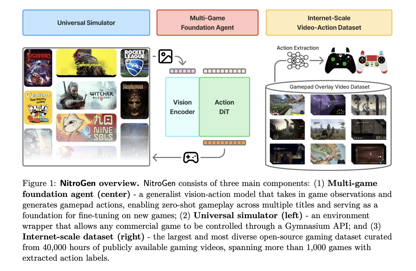
NVIDIA AI research team released NitroGen, an open vision action foundation model for generalist gaming agents that learns to play commercial games directly from pixels and gamepad actions using internet video at scale. NitroGen is trained on 40,000 hours of gameplay across more than 1,000 games and comes with an open dataset, a universal simulator, and a pre trained policy.

Internet scale video action dataset

The NitroGen pipeline starts from publicly available gameplay videos that include input overlays, for example gamepad visualizations that streamers place in a corner of the screen. The research team collects 71,000 hours of raw video with such overlays, then applies quality filtering based on action density, which leaves 55% of the data, about 40,000 hours, spanning more than 1,000 games.

The curated dataset contains 38,739 videos from 818 creators. The distribution covers a wide range of titles. There are 846 games with more than 1 hour of data, 91 games with more than 100 hours, and 15 games with more than 1,000 hours each. Action RPGs account for 34.9 percent of the hours, platformers for 18.4 percent, and action adventure titles for 9.2 percent, with the rest spread across sports, roguelike, racing and other genres.

Action extraction from controller overlays

To recover frame level actions from raw streams, NitroGen uses a three stage action extraction pipeline. First, a template matching module localizes the controller overlay using about 300 controller templates. For each video, the system samples 25 frames and matches SIFT and XFeat features between frames and templates, then estimates an affine transform when at least 20 inliers support a match. This yields a crop of the controller region for all frames.

Second, a SegFormer based hybrid classification segmentation model parses the controller crops. The model takes two consecutive frames concatenated spatially and outputs joystick locations on an 11 by 11 grid plus binary button states. It is trained on 8 million synthetic images rendered with different controller templates, opacities, sizes and compression settings, using AdamW with learning rate 0.0001, weight decay 0.1, and batch size 256.

Third, the pipeline refines joystick positions and filters low activity segments. Joystick coordinates are normalized to the range from −1.0 to 1.0 using the 99th percentile of absolute x and y values to reduce outliers. Chunks where fewer than 50 percent of timesteps have non zero actions are removed, which avoids over predicting the null action during policy training.

A separate benchmark with ground truth controller logs shows that joystick predictions reach an average R² of 0.84 and button frame accuracy reaches 0.96 across major controller families such as Xbox and PlayStation. This validates that automatic annotations are accurate enough for large scale behavior cloning.

Universal simulator and multi game benchmark

NitroGen includes a universal simulator that wraps commercial Windows games in a Gymnasium compatible interface. The wrapper intercepts the game engine system clock to control simulation time and supports frame by frame interaction without modifying game code, for any title that uses the system clock for physics and interactions.

Observations in this benchmark are single RGB frames. Actions are defined as a unified controller space with a 16 dimensional binary vector for gamepad buttons, four d pad buttons, four face buttons, two shoulders, two triggers, two joystick thumb buttons, start and back, plus a 4 dimensional continuous vector for joystick positions, left and right x,y. This unified layout allows direct transfer of one policy across many games.

The evaluation suite covers 10 commercial games and 30 tasks. There are 5 two dimensional games, three side scrollers and two top down roguelikes, and 5 three dimensional games, two open world games, two combat focused action RPGs and one sports title. Tasks fall into 11 combat tasks, 10 navigation tasks, and 9 game specific tasks with custom objectives.

NitroGen model architecture

The NitroGen foundation policy follows the GR00T N1 architecture pattern for embodied agents. It discards the language and state encoders, and keeps a vision encoder plus a single action head. Input is one RGB frame at 256 by 256 resolution. A SigLIP 2 vision transformer encodes this frame into 256 image tokens.

A diffusion transformer, DiT, generates 16 step chunks of future actions. During training, noisy action chunks are embedded by a multilayer perceptron into action tokens, processed by a stack of DiT blocks with self attention and cross attention to visual tokens, then decoded back into continuous action vectors. The training objective is conditional flow matching with 16 denoising steps over each 16 action chunk.

The released checkpoint has 4.93 × 10^8 parameters. The model card describes the output as a 21 by 16 tensor, where 17 dimensions correspond to binary button states and 4 dimensions store two two dimensional joystick vectors, over 16 future timesteps. This representation is consistent with the unified action space, up to reshaping of the joystick components.

Training outcomes and transfer gains

NitroGen is trained purely with large scale behavior cloning on the internet video dataset. There is no reinforcement learning and no reward design in the base model. Image augmentations include random brightness, contrast, saturation, hue, small rotations, and random crops. Training uses AdamW with weight decay 0.001, a warmup stable decay learning rate schedule with constant phase at 0.0001, and an exponential moving average of weights with decay 0.9999.

After pre training on the full dataset, NitroGen 500M already achieves non trivial task completion rates in zero shot evaluation across all games in the benchmark. Average completion rates stay in the range from about 45 percent to 60 percent across combat, navigation and game specific tasks, and across two dimensional and three dimensional games, despite the noise in internet supervision.

For transfer to unseen games, the research team hold out a title, pre train on the remaining data, and then fine tune on the held out game under a fixed data and compute budget. On an isometric roguelike, fine tuning from NitroGen gives an average relative improvement of about 10 percent compared with training from scratch. On a three dimensional action RPG, the average gain is about 25 percent, and for some combat tasks in the low data regime, 30 hours, the relative improvement reaches 52 percent.

Key Takeaways

• NitroGen is a generalist vision action foundation model for games: It maps 256×256 RGB frames directly to standardized gamepad actions and is trained with pure behavior cloning on internet gameplay, without any reinforcement learning.
• The dataset is large scale and automatically labeled from controller overlays: NitroGen uses 40,000 hours of filtered gameplay from 38,739 videos across more than 1,000 games, where frame level actions are extracted from visual controller overlays using a SegFormer based parsing pipeline.
• Unified controller action space enables cross game transfer: Actions are represented in a shared space of about 20 dimensions per timestep, including binary gamepad buttons and continuous joystick vectors, which allows a single policy to be deployed across many commercial Windows games using a universal Gymnasium style simulator.
• Diffusion transformer policy with conditional flow matching: The 4.93 × 10^8 parameter model uses a SigLIP 2 vision encoder plus a DiT based action head trained with conditional flow matching on 16 step action chunks, achieving robust control from noisy web scale data.
• Pretraining on NitroGen improves downstream game performance: When fine tuned on held out titles under the same data and compute budget, NitroGen based initialization yields consistent relative gains, around 10 percent to 25 percent on average and up to 52 percent in low data combat tasks, compared to training from scratch.

Check out the  and . Also, feel free to follow us on  and don’t forget to join our  and Subscribe to . Wait! are you on telegram? 

The post appeared first on .

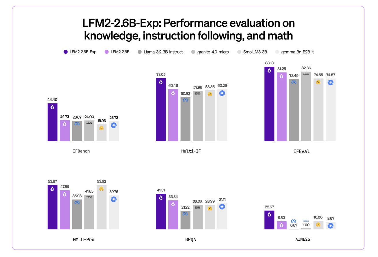
Liquid AI has introduced LFM2-2.6B-Exp, an experimental checkpoint of its LFM2-2.6B language model that is trained with pure reinforcement learning on top of the existing LFM2 stack. The goal is simple, improve instruction following, knowledge tasks, and math for a small 3B class model that still targets on device and edge deployment.

Where LFM2-2.6B-Exp Fits in the LFM2 Family?

LFM2 is the second generation of Liquid Foundation Models. It is designed for efficient deployment on phones, laptops, and other edge devices. Liquid AI describes LFM2 as a hybrid model that combines short range LIV convolution blocks with grouped query attention blocks, controlled by multiplicative gates.

The family includes 4 dense sizes, LFM2-350M, LFM2-700M, LFM2-1.2B, and LFM2-2.6B. All share a context length of 32,768 tokens, a vocabulary size of 65,536, and bfloat16 precision. The 2.6B model uses 30 layers, with 22 convolution layers and 8 attention layers. Each size is trained on a 10 trillion token budget.

LFM2-2.6B is already positioned as a high efficiency model. It reaches 82.41 percent on GSM8K and 79.56 percent on IFEval. This places it ahead of several 3B class models such as Llama 3.2 3B Instruct, Gemma 3 4B it, and SmolLM3 3B on these benchmarks.

LFM2-2.6B-Exp keeps this architecture. It reuses the same tokenization, context window, and hardware profile. The checkpoint focuses only on changing behavior through a reinforcement learning stage.

Pure RL on Top of a Pretrained, Aligned Base

This checkpoint is built on LFM2-2.6B using pure reinforcement learning. It is specifically trained on instruction following, knowledge, and math.

The underlying LFM2 training stack combines several stages. It includes very large scale supervised fine tuning on a mix of downstream tasks and general domains, custom Direct Preference Optimization with length normalization, iterative model merging, and reinforcement learning with verifiable rewards.

But exactly ‘pure reinforcement learning’ means? LFM2-2.6B-Exp starts from the existing LFM2-2.6B checkpoint and then goes through a sequential RL training schedule. It begin with instruction following, then extend RL training to knowledge oriented prompts, math, and a small amount of tool use, without an additional SFT warm up or distillation step in that final phase.

The important point is that LFM2-2.6B-Exp does not change the base architecture or pre training. It changes the policy through an RL stage that uses verifiable rewards, on a targeted set of domains, on top of a model that is already supervised and preference aligned.

Benchmark Signal, Especially On IFBench

Liquid AI team highlights IFBench as the main headline metric. IFBench is an instruction following benchmark that checks how reliably a model follows complex, constrained instructions. On this benchmark, LFM2-2.6B-Exp surpasses DeepSeek R1-0528, which is reported as 263 times larger in parameter count.

LFM2 models provide strong performance across a standard set of benchmarks such as MMLU, GPQA, IFEval, GSM8K, and related suites. The 2.6B base model already competes well in the 3B segment. The RL checkpoint then pushes instruction following and math further, while staying in the same 3B parameter budget.

Architecture and Capabilities that Matters

The architecture uses 10 double gated short range LIV convolution blocks and 6 grouped query attention blocks, arranged in a hybrid stack. This design reduces KV cache cost and keeps inference fast on consumer GPUs and NPUs.

The pre training mixture uses roughly 75 percent English, 20 percent multilingual data, and 5 percent code. The supported languages include English, Arabic, Chinese, French, German, Japanese, Korean, and Spanish.

LFM2 models expose a ChatML like template and native tool use tokens. Tools are described as JSON between dedicated tool list markers. The model then emits Python like calls between tool call markers and reads tool responses between tool response markers. This structure makes the model suitable as the agent core for tool calling stacks without custom prompt engineering.

LFM2-2.6B, and by extension LFM2-2.6B-Exp, is also the only model in the family that enables dynamic hybrid reasoning through special think tokens for complex or multilingual inputs. That capability remains available because the RL checkpoint does not change tokenization or architecture.

Key Takeaways

1. LFM2-2.6B-Exp is an experimental checkpoint of LFM2-2.6B that adds a pure reinforcement learning stage on top of a pretrained, supervised and preference aligned base, targeted at instruction following, knowledge tasks, and math.
2. The LFM2-2.6B backbone uses a hybrid architecture that combines double gated short range LIV convolution blocks and grouped query attention blocks, with 30 layers, 22 convolution layers and 8 attention layers, 32,768 token context length, and a 10 trillion token training budget at 2.6B parameters.
3. LFM2-2.6B already achieves strong benchmark scores in the 3B class, around 82.41 percent on GSM8K and 79.56 percent on IFEval, and the LFM2-2.6B-Exp RL checkpoint further improves instruction following and math performance without changing the architecture or memory profile.
4. Liquid AI reports that on IFBench, an instruction following benchmark, LFM2-2.6B-Exp surpasses DeepSeek R1-0528 even though the latter has many more parameters, which shows a strong performance per parameter for constrained deployment settings.
5. LFM2-2.6B-Exp is released on Hugging Face with open weights under the LFM Open License v1.0 and is supported through Transformers, vLLM, llama.cpp GGUF quantizations, and ONNXRuntime, making it suitable for agentic systems, structured data extraction, retrieval augmented generation, and on device assistants where a compact 3B model is required.

Check out the . Also, feel free to follow us on  and don’t forget to join our  and Subscribe to . Wait! are you on telegram? 

The post appeared first on .

Google has released FunctionGemma, a specialized version of the Gemma 3 270M model that is trained specifically for function calling and designed to run as an edge agent that maps natural language to executable API actions.

But, What is FunctionGemma?

FunctionGemma is a 270M parameter text only transformer based on Gemma 3 270M. It keeps the same architecture as Gemma 3 and is released as an open model under the Gemma license, but the training objective and chat format are dedicated to function calling rather than free form dialogue.

The model is intended to be fine tuned for specific function calling tasks. It is not positioned as a general chat assistant. The primary design goal is to translate user instructions and tool definitions into structured function calls, then optionally summarize tool responses for the user.

From an interface perspective, FunctionGemma is presented as a standard causal language model. Inputs and outputs are text sequences, with an input context of 32K tokens and an output budget of up to 32K tokens per request, shared with the input length.

Architecture and training data

The model uses the Gemma 3 transformer architecture and the same 270M parameter scale as Gemma 3 270M. The training and runtime stack reuse the research and infrastructure used for Gemini, including JAX and ML Pathways on large TPU clusters.

FunctionGemma uses Gemma’s 256K vocabulary, which is optimized for JSON structures and multilingual text. This improves token efficiency for function schemas and tool responses and reduces sequence length for edge deployments where latency and memory are tight.

The model is trained on 6T tokens, with a knowledge cutoff in August 2024. The dataset focuses on two main categories:

• public tool and API definitions
• tool use interactions that include prompts, function calls, function responses and natural language follow up messages that summarize outputs or request clarification

This training signal teaches both syntax, which function to call and how to format arguments, and intent, when to call a function and when to ask for more information.

Conversation format and control tokens

FunctionGemma does not use a free form chat format. It expects a strict conversation template that separates roles and tool related regions. Conversation turns are wrapped with <start_of_turn>role ... <end_of_turn> where roles are typically developer, user or model.

Within those turns, FunctionGemma relies on a fixed set of control token pairs

• <start_function_declaration> and <end_function_declaration> for tool definitions
• <start_function_call> and <end_function_call> for the model’s tool calls
• <start_function_response> and <end_function_response> for serialized tool outputs

These markers let the model distinguish natural language text from function schemas and from execution results. The Hugging Face apply_chat_template API and the official Gemma templates generate this structure automatically for messages and tool lists.

Fine tuning and Mobile Actions performance

Out of the box, FunctionGemma is already trained for generic tool use. However, the official Mobile Actions guide and the model card emphasize that small models reach production level reliability only after task specific fine tuning.

The Mobile Actions demo uses a dataset where each example exposes a small set of tools for Android system operations, for example create a contact, set a calendar event, control the flashlight and map viewing. FunctionGemma learns to map utterances such as ‘Create a calendar event for lunch tomorrow’ or ‘Turn on the flashlight’ to those tools with structured arguments.

On the Mobile Actions evaluation, the base FunctionGemma model reaches 58 percent accuracy on a held out test set. After fine tuning with the public cookbook recipe, accuracy increases to 85 percent.

Edge agents and reference demos

The main deployment target for FunctionGemma is edge agents that run locally on phones, laptops and small accelerators such as NVIDIA Jetson Nano. The small parameter count, 0.3B, and support for quantization allow inference with low memory and low latency on consumer hardware.

Google ships several reference experiences through the Google AI Edge Gallery

• Mobile Actions shows a fully offline assistant style agent for device control using FunctionGemma fine tuned on the Mobile Actions dataset and deployed on device.
• Tiny Garden is a voice controlled game where the model decomposes commands such as “Plant sunflowers in the top row and water them” into domain specific functions like plant_seed and water_plots with explicit grid coordinates.
• FunctionGemma Physics Playground runs entirely in the browser using Transformers.js and lets users solve physics puzzles via natural language instructions that the model converts into simulation actions.

These demos validate that a 270M parameter function caller can support multi step logic on device without server calls, given appropriate fine tuning and tool interfaces.

Key Takeaways

1. FunctionGemma is a 270M parameter, text only variant of Gemma 3 that is trained specifically for function calling, not for open ended chat, and is released as an open model under the Gemma terms of use.
2. The model keeps the Gemma 3 transformer architecture and 256k token vocabulary, supports 32k tokens per request shared between input and output, and is trained on 6T tokens.
3. FunctionGemma uses a strict chat template with <start_of_turn>role ... <end_of_turn> and dedicated control tokens for function declarations, function calls and function responses, which is required for reliable tool use in production systems.
4. On the Mobile Actions benchmark, accuracy improves from 58 percent for the base model to 85 percent after task specific fine tuning, showing that small function callers need domain data more than prompt engineering.
5. The 270M scale and quantization support let FunctionGemma run on phones, laptops and Jetson class devices, and the model is already integrated into ecosystems such as Hugging Face, Vertex AI, LM Studio and edge demos like Mobile Actions, Tiny Garden and the Physics Playground.

Check out the  and  Also, feel free to follow us on  and don’t forget to join our  and Subscribe to . Wait! are you on telegram? 

The post appeared first on .

In this tutorial, we dive into the cutting edge of Agentic AI by building a “Zettelkasten” memory system, a “living” architecture that organizes information much like the human brain. We move beyond standard retrieval methods to construct a dynamic knowledge graph where an agent autonomously decomposes inputs into atomic facts, links them semantically, and even “sleeps” to consolidate memories into higher-order insights. Using Google’s Gemini, we implement a robust solution that addresses real-world API constraints, ensuring our agent stores data and also actively understands the evolving context of our projects. Check out the .

!pip install -q -U google-generativeai networkx pyvis scikit-learn numpy


import os
import json
import uuid
import time
import getpass
import random
import networkx as nx
import numpy as np
import google.generativeai as genai
from dataclasses import dataclass, field
from typing import List
from sklearn.metrics.pairwise import cosine_similarity
from IPython.display import display, HTML
from pyvis.network import Network
from google.api_core import exceptions


def retry_with_backoff(func, *args, **kwargs):
   max_retries = 5
   base_delay = 5
  
   for attempt in range(max_retries):
       try:
           return func(*args, **kwargs)
       except exceptions.ResourceExhausted:
           wait_time = base_delay * (2 ** attempt) + random.uniform(0, 1)
           print(f"    Quota limit hit. Cooling down for {wait_time:.1f}s...")
           time.sleep(wait_time)
       except Exception as e:
           if "429" in str(e):
               wait_time = base_delay * (2 ** attempt) + random.uniform(0, 1)
               print(f"    Quota limit hit (HTTP 429). Cooling down for {wait_time:.1f}s...")
               time.sleep(wait_time)
           else:
               print(f"    Unexpected Error: {e}")
               return None
   print("    Max retries reached.")
   return None


print("Enter your Google AI Studio API Key (Input will be hidden):")
API_KEY = getpass.getpass()


genai.configure(api_key=API_KEY)
MODEL_NAME = "gemini-2.5-flash" 
EMBEDDING_MODEL = "models/text-embedding-004"


print(f" API Key configured. Using model: {MODEL_NAME}")

We begin by importing essential libraries for graph management and AI model interaction, while also securing our API key input. Crucially, we define a robust retry_with_backoff function that automatically handles rate limit errors, ensuring our agent gracefully pauses and recovers when the API quota is exceeded during heavy processing. Check out the .

@dataclass
class MemoryNode:
   id: str
   content: str
   type: str
   embedding: List[float] = field(default_factory=list)
   timestamp: int = 0


class RobustZettelkasten:
   def __init__(self):
       self.graph = nx.Graph()
       self.model = genai.GenerativeModel(MODEL_NAME)
       self.step_counter = 0


   def _get_embedding(self, text):
       result = retry_with_backoff(
           genai.embed_content,
           model=EMBEDDING_MODEL,
           content=text
       )
       return result['embedding'] if result else [0.0] * 768

We define the fundamental MemoryNode structure to hold our content, types, and vector embeddings in an organized data class. We then initialize the main RobustZettelkasten class, establishing the network graph and configuring the Gemini embedding model that serves as the backbone of our semantic search capabilities. Check out the .

def _atomize_input(self, text):
       prompt = f"""
       Break the following text into independent atomic facts.
       Output JSON: {{ "facts": ["fact1", "fact2"] }}
       Text: "{text}"
       """
       response = retry_with_backoff(
           self.model.generate_content,
           prompt,
           generation_config={"response_mime_type": "application/json"}
       )
       try:
           return json.loads(response.text).get("facts", []) if response else [text]
       except:
           return [text]


   def _find_similar_nodes(self, embedding, top_k=3, threshold=0.45):
       if not self.graph.nodes: return []
      
       nodes = list(self.graph.nodes(data=True))
       embeddings = [n[1]['data'].embedding for n in nodes]
       valid_embeddings = [e for e in embeddings if len(e) > 0]
      
       if not valid_embeddings: return []


       sims = cosine_similarity([embedding], embeddings)[0]
       sorted_indices = np.argsort(sims)[::-1]
      
       results = []
       for idx in sorted_indices[:top_k]:
           if sims[idx] > threshold:
               results.append((nodes[idx][0], sims[idx]))
       return results


   def add_memory(self, user_input):
       self.step_counter += 1
       print(f"n [Step {self.step_counter}] Processing: "{user_input}"")
      
       facts = self._atomize_input(user_input)
      
       for fact in facts:
           print(f"   -> Atom: {fact}")
           emb = self._get_embedding(fact)
           candidates = self._find_similar_nodes(emb)
          
           node_id = str(uuid.uuid4())[:6]
           node = MemoryNode(id=node_id, content=fact, type='fact', embedding=emb, timestamp=self.step_counter)
           self.graph.add_node(node_id, data=node, title=fact, label=fact[:15]+"...")
          
           if candidates:
               context_str = "n".join([f"ID {c[0]}: {self.graph.nodes[c[0]]['data'].content}" for c in candidates])
               prompt = f"""
               I am adding: "{fact}"
               Existing Memory:
               {context_str}
              
               Are any of these directly related? If yes, provide the relationship label.
               JSON: {{ "links": [{{ "target_id": "ID", "rel": "label" }}] }}
               """
               response = retry_with_backoff(
                   self.model.generate_content,
                   prompt,
                   generation_config={"response_mime_type": "application/json"}
               )
              
               if response:
                   try:
                       links = json.loads(response.text).get("links", [])
                       for link in links:
                           if self.graph.has_node(link['target_id']):
                               self.graph.add_edge(node_id, link['target_id'], label=link['rel'])
                               print(f"       Linked to {link['target_id']} ({link['rel']})")
                   except:
                       pass
          
           time.sleep(1)

We construct an ingestion pipeline that decomposes complex user inputs into atomic facts to prevent information loss. We immediately embed these facts and use our agent to identify and create semantic links to existing nodes, effectively building a knowledge graph in real time that mimics associative memory. Check out the .

def consolidate_memory(self):
       print(f"n [Consolidation Phase] Reflecting...")
       high_degree_nodes = [n for n, d in self.graph.degree() if d >= 2]
       processed_clusters = set()


       for main_node in high_degree_nodes:
           neighbors = list(self.graph.neighbors(main_node))
           cluster_ids = tuple(sorted([main_node] + neighbors))
          
           if cluster_ids in processed_clusters: continue
           processed_clusters.add(cluster_ids)
          
           cluster_content = [self.graph.nodes[n]['data'].content for n in cluster_ids]
          
           prompt = f"""
           Generate a single high-level insight summary from these facts.
           Facts: {json.dumps(cluster_content)}
           JSON: {{ "insight": "Your insight here" }}
           """
           response = retry_with_backoff(
               self.model.generate_content,
               prompt,
               generation_config={"response_mime_type": "application/json"}
           )
          
           if response:
               try:
                   insight_text = json.loads(response.text).get("insight")
                   if insight_text:
                       insight_id = f"INSIGHT-{uuid.uuid4().hex[:4]}"
                       print(f"    Insight: {insight_text}")
                       emb = self._get_embedding(insight_text)
                      
                       insight_node = MemoryNode(id=insight_id, content=insight_text, type='insight', embedding=emb)
                       self.graph.add_node(insight_id, data=insight_node, title=f"INSIGHT: {insight_text}", label="INSIGHT", color="#ff7f7f")
                       self.graph.add_edge(insight_id, main_node, label="abstracted_from")
               except:
                   continue
           time.sleep(1)


   def answer_query(self, query):
       print(f"n Querying: "{query}"")
       emb = self._get_embedding(query)
       candidates = self._find_similar_nodes(emb, top_k=2)
      
       if not candidates:
           print("No relevant memory found.")
           return


       relevant_context = set()
       for node_id, score in candidates:
           node_content = self.graph.nodes[node_id]['data'].content
           relevant_context.add(f"- {node_content} (Direct Match)")
           for n1 in self.graph.neighbors(node_id):
               rel = self.graph[node_id][n1].get('label', 'related')
               content = self.graph.nodes[n1]['data'].content
               relevant_context.add(f"  - linked via '{rel}' to: {content}")
              
       context_text = "n".join(relevant_context)
       prompt = f"""
       Answer based ONLY on context.
       Question: {query}
       Context:
       {context_text}
       """
       response = retry_with_backoff(self.model.generate_content, prompt)
       if response:
           print(f" Agent Answer:n{response.text}")

We implement the cognitive functions of our agent, enabling it to “sleep” and consolidate dense memory clusters into higher-order insights. We also define the query logic that traverses these connected paths, allowing the agent to reason across multiple hops in the graph to answer complex questions. Check out the .

def show_graph(self):
       try:
           net = Network(notebook=True, cdn_resources='remote', height="500px", width="100%", bgcolor='#222222', font_color='white')
           for n, data in self.graph.nodes(data=True):
               color = "#97c2fc" if data['data'].type == 'fact' else "#ff7f7f"
               net.add_node(n, label=data.get('label', ''), title=data['data'].content, color=color)
           for u, v, data in self.graph.edges(data=True):
               net.add_edge(u, v, label=data.get('label', ''))
           net.show("memory_graph.html")
           display(HTML("memory_graph.html"))
       except Exception as e:
           print(f"Graph visualization error: {e}")


brain = RobustZettelkasten()


events = [
   "The project 'Apollo' aims to build a dashboard for tracking solar panel efficiency.",
   "We chose React for the frontend because the team knows it well.",
   "The backend must be Python to support the data science libraries.",
   "Client called. They are unhappy with React performance on low-end devices.",
   "We are switching the frontend to Svelte for better performance."
]


print("--- PHASE 1: INGESTION ---")
for event in events:
   brain.add_memory(event)
   time.sleep(2)


print("--- PHASE 2: CONSOLIDATION ---")
brain.consolidate_memory()


print("--- PHASE 3: RETRIEVAL ---")
brain.answer_query("What is the current frontend technology for Apollo and why?")


print("--- PHASE 4: VISUALIZATION ---")
brain.show_graph()

We wrap up by adding a visualization method that generates an interactive HTML graph of our agent’s memory, allowing us to inspect the nodes and edges. Finally, we execute a test scenario involving a project timeline to verify that our system correctly links concepts, generates insights, and retrieves the right context.

In conclusion, we now have a fully functional “Living Memory” prototype that transcends simple database storage. By enabling our agent to actively link related concepts and reflect on its experiences during a “consolidation” phase, we solve the critical problem of fragmented context in long-running AI interactions. This system demonstrates that true intelligence requires processing power and a structured, evolving memory, marking the way for us to build more capable, personalized autonomous agents.

Check out the . Also, feel free to follow us on  and don’t forget to join our  and Subscribe to . Wait! are you on telegram? 

The post appeared first on .