December 4, 2025
Can AI Look at Your Retina and Diagnose Alzheimer’s? Eric Topol Hopes So
The author of Super Agers believes AI could bring big changes to the world of medicine.
 December 4, 2025
The author of Super Agers believes AI could bring big changes to the world of medicine.
 December 4, 2025
The Trump administration might think regulation is killing the AI industry, but Anthropic president Daniela Amodei disagrees.
 December 4, 2025
In this episode of Uncanny Valley, we talk to writer Evan Ratliff about how he created a small startup made entirely of AI employees—and what his findings reveal about the reality of an agentic future.
 December 4, 2025
The Wicked: For Good director says being able to improvise on set allows for the kind of moments that are hard for machines to make.
 December 4, 2025
Lisa Su leads Nvidia’s biggest rival in the AI chip market. When asked at WIRED’s Big Interview event if AI is a bubble, company said “Emphatically, from my perspective, no.”
 December 4, 2025
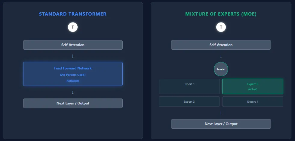
MoE models contain far more parameters than Transformers, yet they can run faster at inference. How is that possible?
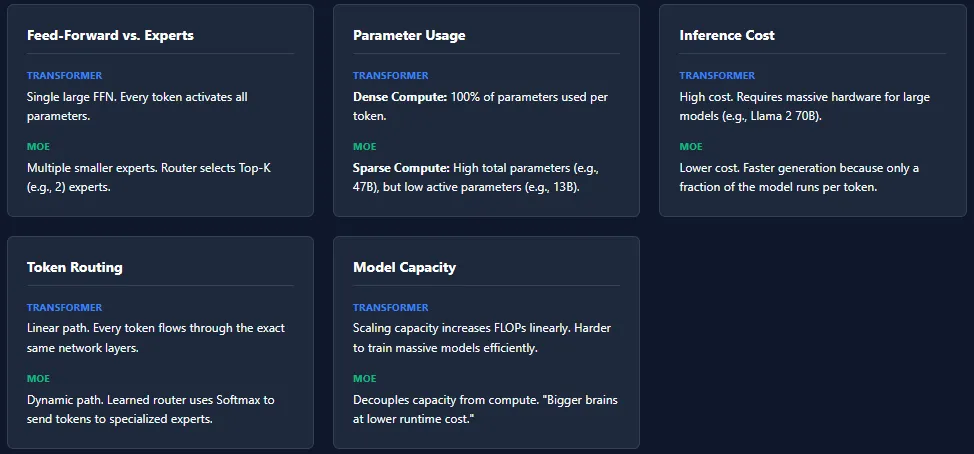
Transformers and Mixture of Experts (MoE) models share the same backbone architecture—self-attention layers followed by feed-forward layers—but they differ fundamentally in how they use parameters and compute.
While MoE architectures offer massive capacity with lower inference cost, they introduce several training challenges. The most common issue is expert collapse, where the router repeatedly selects the same experts, leaving others under-trained.
Load imbalance is another challenge—some experts may receive far more tokens than others, leading to uneven learning. To address this, MoE models rely on techniques like noise injection in routing, Top-K masking, and expert capacity limits.
These mechanisms ensure all experts stay active and balanced, but they also make MoE systems more complex to train compared to standard Transformers.
The post appeared first on .
 December 4, 2025
In this tutorial, we build an advanced meta-cognitive control agent that learns how to regulate its own depth of thinking. We treat reasoning as a spectrum, ranging from fast heuristics to deep chain-of-thought to precise tool-like solving, and we train a neural meta-controller to decide which mode to use for each task. By optimizing the trade-off between accuracy, computation cost, and a limited reasoning budget, we explore how an agent can monitor its internal state and adapt its reasoning strategy in real time. Through each snippet, we experiment, observe patterns, and understand how meta-cognition emerges when an agent learns to think about its own thinking. Check out the .
import random
import numpy as np
import torch
import torch.nn as nn
import torch.optim as optim


OPS = ['+', '*']


def make_task():
   op = random.choice(OPS)
   if op == '+':
       a, b = random.randint(1, 99), random.randint(1, 99)
   else:
       a, b = random.randint(2, 19), random.randint(2, 19)
   return a, b, op


def true_answer(a, b, op):
   return a + b if op == '+' else a * b


def true_difficulty(a, b, op):
   if op == '+' and a <= 30 and b <= 30:
       return 0
   if op == '*' and a <= 10 and b <= 10:
       return 1
   return 2


def heuristic_difficulty(a, b, op):
   score = 0
   if op == '*':
       score += 0.6
   score += max(a, b) / 100.0
   return min(score, 1.0)


def fast_heuristic(a, b, op):
   if op == '+':
       base = a + b
       noise = random.choice([-2, -1, 0, 0, 0, 1, 2, 3])
   else:
       base = int(0.8 * a * b)
       noise = random.choice([-5, -3, 0, 0, 2, 5, 8])
   return base + noise, 0.5


def deep_chain_of_thought(a, b, op, verbose=False):
   if op == '+':
       x, y = a, b
       carry = 0
       pos = 1
       result = 0
       step = 0
       while x > 0 or y > 0 or carry:
           dx, dy = x % 10, y % 10
           s = dx + dy + carry
           carry, digit = divmod(s, 10)
           result += digit * pos
           x //= 10; y //= 10; pos *= 10
           step += 1
   else:
       result = 0
       step = 0
       for i, d in enumerate(reversed(str(b))):
           row = a * int(d) * (10 ** i)
           result += row
           step += 1
   return result, max(2.0, 0.4 * step)


def tool_solver(a, b, op):
   return eval(f"{a}{op}{b}"), 1.2


ACTION_NAMES = ["fast", "deep", "tool"]
We set up the world our meta-agent operates in. We generate arithmetic tasks, define ground-truth answers, estimate difficulty, and implement three different reasoning modes. As we run it, we observe how each solver behaves differently in terms of accuracy and computational cost, which form the foundation of the agent’s decision space. Check out the .
def encode_state(a, b, op, rem_budget, error_ema, last_action):
   a_n = a / 100.0
   b_n = b / 100.0
   op_plus = 1.0 if op == '+' else 0.0
   op_mul = 1.0 - op_plus
   diff_hat = heuristic_difficulty(a, b, op)
   rem_n = rem_budget / MAX_BUDGET
   last_onehot = [0.0, 0.0, 0.0]
   if last_action is not None:
       last_onehot[last_action] = 1.0
   feats = [
       a_n, b_n, op_plus, op_mul,
       diff_hat, rem_n, error_ema
   ] + last_onehot
   return torch.tensor(feats, dtype=torch.float32, device=device)


STATE_DIM = 10
N_ACTIONS = 3


class PolicyNet(nn.Module):
   def __init__(self, state_dim, hidden=48, n_actions=3):
       super().__init__()
       self.net = nn.Sequential(
           nn.Linear(state_dim, hidden),
           nn.Tanh(),
           nn.Linear(hidden, hidden),
           nn.Tanh(),
           nn.Linear(hidden, n_actions)
       )
   def forward(self, x):
       return self.net(x)


policy = PolicyNet(STATE_DIM, hidden=48, n_actions=N_ACTIONS).to(device)
optimizer = optim.Adam(policy.parameters(), lr=3e-3)
We encode each task into a structured state that captures operands, operation type, predicted difficulty, remaining budget, and recent performance. We then define a neural policy network that maps this state to a probability distribution over actions. As we work through it, we see how the policy becomes the core mechanism through which the agent learns to regulate its thinking. Check out the .
GAMMA = 0.98
COST_PENALTY = 0.25
MAX_BUDGET = 25.0
EPISODES = 600
STEPS_PER_EP = 20
ERROR_EMA_DECAY = 0.9


def run_episode(train=True):
   log_probs = []
   rewards = []
   info = []
   rem_budget = MAX_BUDGET
   error_ema = 0.0
   last_action = None


   for _ in range(STEPS_PER_EP):
       a, b, op = make_task()
       state = encode_state(a, b, op, rem_budget, error_ema, last_action)
       logits = policy(state)
       dist = torch.distributions.Categorical(logits=logits)
       action = dist.sample() if train else torch.argmax(logits)
       act_idx = int(action.item())


       if act_idx == 0:
           pred, cost = fast_heuristic(a, b, op)
       elif act_idx == 1:
           pred, cost = deep_chain_of_thought(a, b, op, verbose=False)
       else:
           pred, cost = tool_solver(a, b, op)


       correct = (pred == true_answer(a, b, op))
       acc_reward = 1.0 if correct else 0.0
       budget_penalty = 0.0


       rem_budget -= cost
       if rem_budget < 0:
           budget_penalty = -1.5 * (abs(rem_budget) / MAX_BUDGET)


       step_reward = acc_reward - COST_PENALTY * cost + budget_penalty
       rewards.append(step_reward)


       if train:
           log_probs.append(dist.log_prob(action))


       err = 0.0 if correct else 1.0
       error_ema = ERROR_EMA_DECAY * error_ema + (1 - ERROR_EMA_DECAY) * err
       last_action = act_idx


       info.append({
           "correct": correct,
           "cost": cost,
           "difficulty": true_difficulty(a, b, op),
           "action": act_idx
       })


   if train:
       returns = []
       G = 0.0
       for r in reversed(rewards):
           G = r + GAMMA * G
           returns.append(G)
       returns = list(reversed(returns))
       returns_t = torch.tensor(returns, dtype=torch.float32, device=device)
       baseline = returns_t.mean()
       adv = returns_t - baseline
       loss = -(torch.stack(log_probs) * adv).mean()
       optimizer.zero_grad()
       loss.backward()
       optimizer.step()


   return rewards, info
We implement the heart of learning using the REINFORCE policy gradient algorithm. We run multi-step episodes, collect log-probabilities, accumulate rewards, and compute returns. As we execute this part, we watch the meta-controller adjust its strategy by reinforcing decisions that balance accuracy with cost. Check out the .
print("Training meta-cognitive controller...")
for ep in range(EPISODES):
   rewards, _ = run_episode(train=True)
   if (ep + 1) % 100 == 0:
       print(f" episode {ep+1:4d} | avg reward {np.mean(rewards):.3f}")


def evaluate(n_episodes=50):
   all_actions = {0: [0,0,0], 1: [0,0,0], 2: [0,0,0]}
   stats = {0: {"n":0,"acc":0,"cost":0},
            1: {"n":0,"acc":0,"cost":0},
            2: {"n":0,"acc":0,"cost":0}}


   for _ in range(n_episodes):
       _, info = run_episode(train=False)
       for step in info:
           d = step["difficulty"]
           a_idx = step["action"]
           all_actions[d][a_idx] += 1
           stats[d]["n"] += 1
           stats[d]["acc"] += 1 if step["correct"] else 0
           stats[d]["cost"] += step["cost"]


   for d in [0,1,2]:
       if stats[d]["n"] == 0:
           continue
       n = stats[d]["n"]
       print(f"Difficulty {d}:")
       print(" action counts [fast, deep, tool]:", all_actions[d])
       print(" accuracy:", stats[d]["acc"]/n)
       print(" avg cost:", stats[d]["cost"]/n)
       print()


print("Policy behavior by difficulty:")
evaluate()
We train the meta-cognitive agent over hundreds of episodes and evaluate its behavior across difficulty levels. We observe how the policy evolves, using fast heuristics for simple tasks while resorting to deeper reasoning for harder ones. As we analyze the outputs, we understand how training shapes the agent’s reasoning choices. Check out the .
print("nExample hard task with meta-selected thinking mode:")
a, b, op = 47, 18, '*'
state = encode_state(a, b, op, MAX_BUDGET, 0.3, None)
with torch.no_grad():
   logits = policy(state)
   act = int(torch.argmax(logits).item())


print(f"Task: {a} {op} {b}")
print("Chosen mode:", ACTION_NAMES[act])


if act == 1:
   pred, cost = deep_chain_of_thought(a, b, op, verbose=True)
elif act == 0:
   pred, cost = fast_heuristic(a, b, op)
   print("Fast heuristic:", pred)
else:
   pred, cost = tool_solver(a, b, op)
   print("Tool solver:", pred)


print("True:", true_answer(a,b,op), "| cost:", cost)
We inspect a detailed reasoning trace for a hard example chosen by the trained policy. We see the agent confidently pick a mode and walk through the reasoning steps, allowing us to witness its meta-cognitive behavior in action. As we test different tasks, we appreciate how the model adapts its thinking based on context.
In conclusion, we have seen how a neural controller can learn to dynamically choose the most effective reasoning pathway based on the task’s difficulty and the constraints of the moment. We observe how the agent gradually discovers when quick heuristics are sufficient, when deeper reasoning is necessary, and when calling a precise solver is worth the cost. Through this process, we experience how metacognitive control transforms decision-making, leading to more efficient and adaptable reasoning systems.
Check out the . Feel free to check out our . Also, feel free to follow us on and don’t forget to join our and Subscribe to . Wait! are you on telegram?
The post appeared first on .
 December 4, 2025
The diverging path of China’s two leading AI players shows where the country’s artificial intelligence industry is headed.
 December 4, 2025
Zanskar uses AI to identify hidden geothermal systems—and claims it has found one that could fuel a power plant, the first such discovery by industry in decades.
 December 3, 2025
The Chinese video game giant Tencent is now building some of the world’s best 3D AI models. This could have implications far outside game design.