AI Tools & Reviews

What comes after Transformers? Google Research is proposing a new way to give sequence models usable long term memory with Titans and MIRAS, while keeping training parallel and inference close to linear.

Titans is a concrete architecture that adds a deep neural memory to a Transformer style backbone. MIRAS is a general framework that views most modern sequence models as instances of online optimization over an associative memory.

Why Titans and MIRAS?

Standard Transformers use attention over a key value cache. This gives strong in context learning, but cost grows quadratically with context length, so practical context is limited even with FlashAttention and other kernel tricks.

Efficient linear recurrent neural networks and state space models such as Mamba-2 compress the history into a fixed size state, so cost is linear in sequence length. However, this compression loses information in very long sequences, which hurts tasks such as genomic modeling and extreme long context retrieval.

Titans and MIRAS combine these ideas. Attention acts as a precise short term memory on the current window. A separate neural module provides long term memory, learns at test time, and is trained so that its dynamics are parallelizable on accelerators.

Titans, a neural long term memory that learns at test time

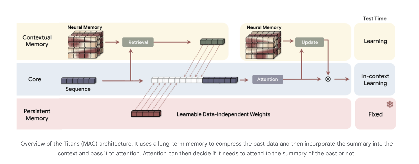
The introduces a neural long term memory module that is itself a deep multi layer perceptron rather than a vector or matrix state. Attention is interpreted as short term memory, since it only sees a limited window, while the neural memory acts as persistent long term memory.

For each token, Titans defines an associative memory loss

ℓ(Mₜ₋₁; kₜ, vₜ) = ‖Mₜ₋₁(kₜ) − vₜ‖²

where Mₜ₋₁ is the current memory, kₜ is the key and vₜ is the value. The gradient of this loss with respect to the memory parameters is the “surprise metric”. Large gradients correspond to surprising tokens that should be stored, small gradients correspond to expected tokens that can be mostly ignored.

The memory parameters are updated at test time by gradient descent with momentum and weight decay, which together act as a retention gate and forgetting mechanism.To keep this online optimization efficient, the research paper shows how to compute these updates with batched matrix multiplications over sequence chunks, which preserves parallel training across long sequences.

Architecturally, Titans uses three memory branches in the backbone, often instanced in the Titans MAC variant:

• a core branch that performs standard in context learning with attention
• a contextual memory branch that learns from the recent sequence
• a persistent memory branch with fixed weights that encodes pretraining knowledge

The long term memory compresses past tokens into a summary, which is then passed as extra context into attention. Attention can choose when to read that summary.

Experimental results for Titans

On language modeling and commonsense reasoning benchmarks such as C4, WikiText and HellaSwag, Titans architectures outperform state of the art linear recurrent baselines Mamba-2 and Gated DeltaNet and Transformer++ models of comparable size. The Google research attribute this to the higher expressive power of deep memory and its ability to maintain performance as context length grows. Deep neural memories with the same parameter budget but higher depth give consistently lower perplexity.

For extreme long context recall, the research team uses the BABILong benchmark, where facts are distributed across very long documents. Titans outperforms all baselines, including very large models such as GPT-4, while using many fewer parameters, and scales to context windows beyond 2,000,000 tokens.

The research team reports that Titans keeps efficient parallel training and fast linear inference. Neural memory alone is slightly slower than the fastest linear recurrent models, but hybrid Titans layers with Sliding Window Attention remain competitive on throughput while improving accuracy.

MIRAS, a unified framework for sequence models as associative memory

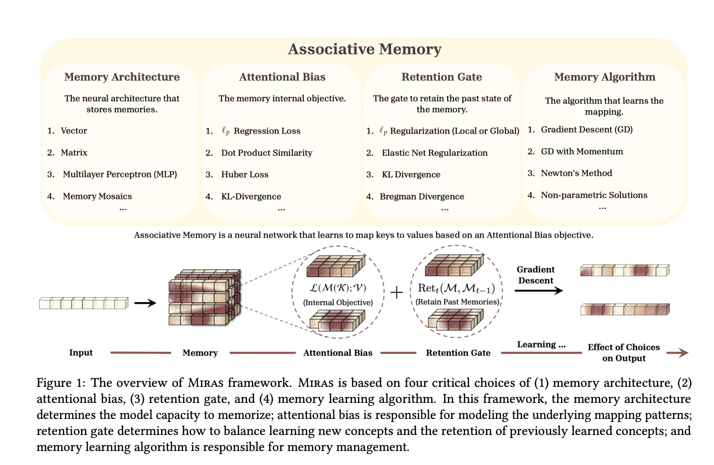
The MIRAS research paper, ,” generalizes this view. It observes that modern sequence models can be seen as associative memories that map keys to values while balancing learning and forgetting.

MIRAS defines any sequence model through four design choices:

1. Memory structure for example a vector, linear map, or MLP
2. Attentional bias the internal loss that defines what similarities the memory cares about
3. Retention gate the regularizer that keeps the memory close to its past state
4. Memory algorithm the online optimization rule, often gradient descent with momentum

Using this lens, MIRAS recovers several families:

• Hebbian style linear recurrent models and RetNet as dot product based associative memories
• Delta rule models such as DeltaNet and Gated DeltaNet as MSE based memories with value replacement and specific retention gates
• Titans LMM as a nonlinear MSE based memory with local and global retention optimized by gradient descent with momentum

Crucially, MIRAS then moves beyond the usual MSE or dot product objectives. The research team constructs new attentional biases based on Lₚ norms, robust Huber loss and robust optimization, and new retention gates based on divergences over probability simplices, elastic net regularization and Bregman divergence.

From this design space, the research team instantiate three attention free models:

• Moneta uses a 2 layer MLP memory with Lₚ attentional bias and a hybrid retention gate based on generalized norms
• Yaad uses the same MLP memory with Huber loss attentional bias and a forget gate related to Titans
• Memora uses regression loss as attentional bias and a KL divergence based retention gate over a probability simplex style memory.

These MIRAS variants replace attention blocks in a Llama style backbone, use depthwise separable convolutions in the Miras layer, and can be combined with Sliding Window Attention in hybrid models. Training remains parallel by chunking sequences and computing gradients with respect to the memory state from the previous chunk.

In research experiments, Moneta, Yaad and Memora match or surpass strong linear recurrent models and Transformer++ on language modeling, commonsense reasoning and recall intensive tasks, while maintaining linear time inference.

Key Takeaways

1. Titans introduces a deep neural long term memory that learns at test time, using gradient descent on an L2 associative memory loss so the model selectively stores only surprising tokens while keeping updates parallelizable on accelerators.
2. Titans combines attention with neural memory for long context, using branches like core, contextual memory and persistent memory so attention handles short range precision and the neural module maintains information over sequences beyond 2,000,000 tokens.
3. Titans outperforms strong linear RNNs and Transformer++ baselines, including Mamba-2 and Gated DeltaNet, on language modeling and commonsense reasoning benchmarks at comparable parameter scales, while staying competitive on throughput.
4. On extreme long context recall benchmarks such as BABILong, Titans achieves higher accuracy than all baselines, including larger attention models such as GPT 4, while using fewer parameters and still enabling efficient training and inference.
5. MIRAS provides a unifying framework for sequence models as associative memories, defining them by memory structure, attentional bias, retention gate and optimization rule, and yields new attention free architectures such as Moneta, Yaad and Memora that match or surpass linear RNNs and Transformer++ on long context and reasoning tasks.

Check out the . Feel free to check out our . Also, feel free to follow us on  and don’t forget to join our  and Subscribe to . Wait! are you on telegram? 

The post appeared first on .

Google is closing an old gap between Kaggle and Colab. Colab now has a built in Data Explorer that lets you search Kaggle datasets, models and competitions directly inside a notebook, then pull them in through KaggleHub without leaving the editor.

What Colab Data Explorer actually ships?

recently where they describe a panel in the Colab notebook editor that connects to Kaggle search.

From this panel you can:

1. Search Kaggle datasets, models and competitions
2. Access the feature from the left toolbar in Colab
3. Use integrated filters to refine the results, for example by resource type or relevance

The Colab Data Explorer lets you search Kaggle datasets, models and competitions directly from a Colab notebook and that you can import data with a KaggleHub code snippet and integrated filters.

The old Kaggle to Colab pipeline was all setup work

Before this launch, most workflows that pulled Kaggle data into Colab followed a fixed sequence.

You created a Kaggle account, generated an API token, downloaded the kaggle.json credentials file, uploaded that file into the Colab runtime, set environment variables and then used the Kaggle API or command line interface to download datasets.

The steps were well documented and reliable. They were also mechanical and easy to misconfigure, especially for beginners who had to debug missing credentials or incorrect paths before they could even run pandas.read_csv on a file. Many tutorials exist only to explain this setup.

Colab Data Explorer does not remove the need for Kaggle credentials. It changes how you reach Kaggle resources and how much code you must write before you can start analysis.

KaggleHub is the integration layer

is a Python library that provides a simple interface to Kaggle datasets, models and notebook outputs from Python environments.

The key properties, which matter for Colab users, are:

1. KaggleHub works in Kaggle notebooks and in external environments such as local Python and Colab
2. It authenticates using existing Kaggle API credentials when needed
3. It exposes resource centric functions such as model_download and dataset_download which take Kaggle identifiers and return paths or objects in the current environment

Colab Data Explorer uses this library as the loading mechanism. When you select a dataset or model in the panel, Colab shows a KaggleHub code snippet that you run inside the notebook to access that resource.

Once the snippet runs, the data is available in the Colab runtime. You can then read it with pandas, train models with PyTorch or TensorFlow or plug it into evaluation code, just as you would with any local files or data objects.

The post appeared first on .

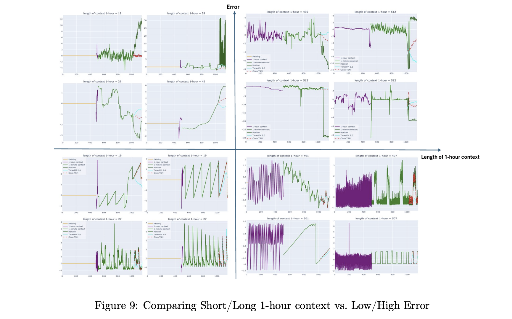
Cisco and Splunk have introduced the Cisco Time Series Model, a univariate zero shot time series foundation model designed for observability and security metrics. It is released as an open weight checkpoint on Hugging Face under an Apache 2.0 license, and it targets forecasting workloads without task specific fine tuning. The model extends TimesFM 2.0 with an explicit multiresolution architecture that fuses coarse and fine history in one context window.

Why observability needs multiresolution context?

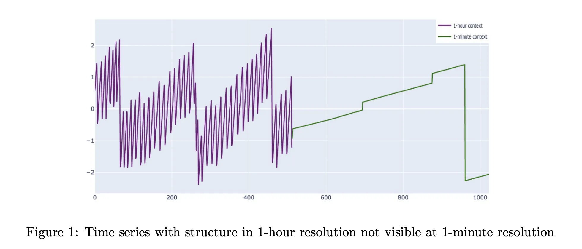
Production metrics are not simple single scale signals. Weekly patterns, long term growth and saturation are visible only at coarse resolutions. Saturation events, traffic spikes and incident dynamics show up at 1 minute or 5 minute resolution. The common time series foundation models work at a single resolution with context windows between 512 and 4096 points, while TimesFM 2.5 extends this to 16384 points. For 1 minute data this still covers at most a couple of weeks and often less.

This is a problem in observability where data platforms often retain only old data in aggregated form. Fine grained samples expire and survive only as 1 hour rollups. Cisco Time Series Model is built for this storage pattern. It treats coarse history as a first class input that improves forecasts at the fine resolution. The architecture operates directly on a multiresolution context instead of pretending that all inputs live on a single grid.

Multiresolution input and forecasting objective

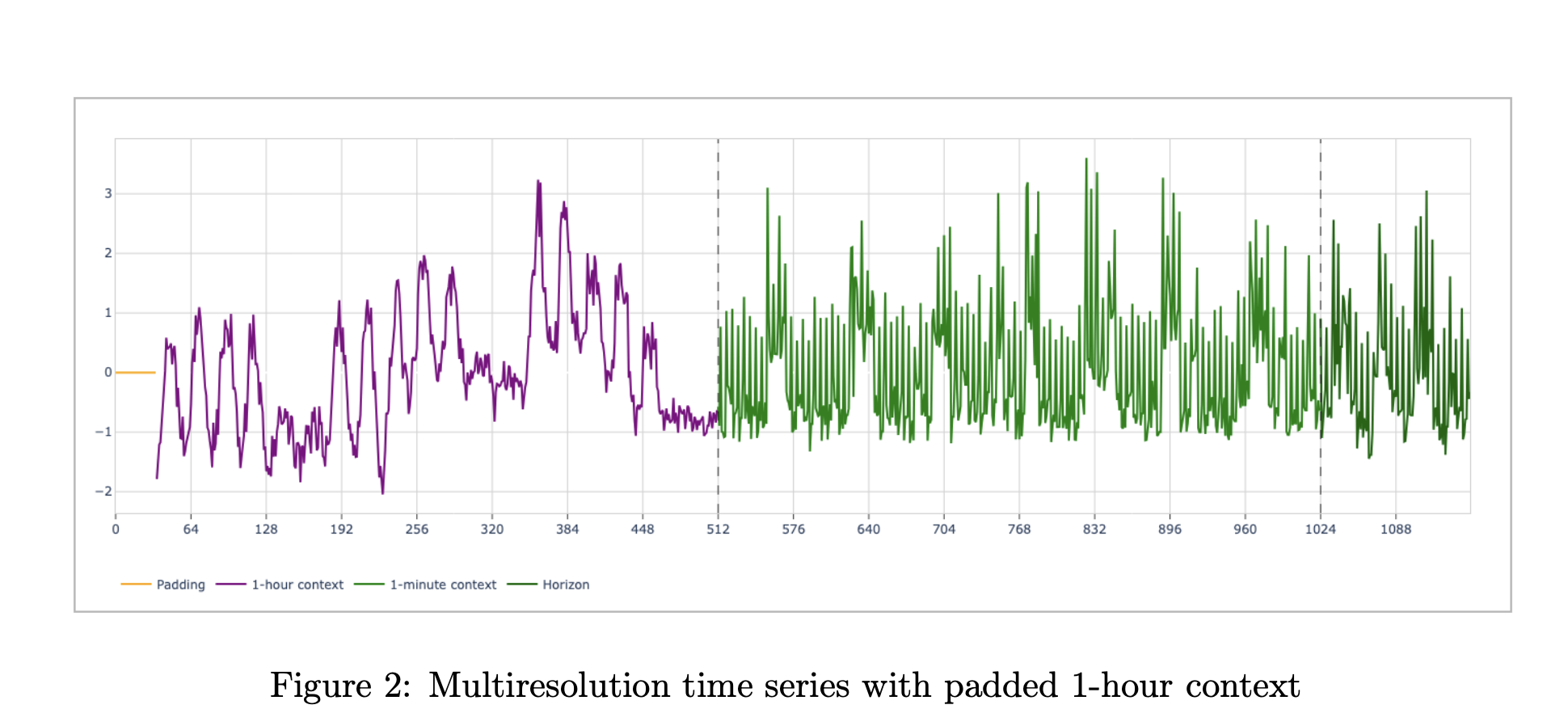
Formally, the model consumes a pair of contexts, (x_c, x_f). The coarse context (x_c) and the fine context (x_f) each have length up to 512. The spacing of (x_c) is fixed at 60 times the spacing of (x_f). A typical observability setup uses 512 hours of 1 hour aggregates and 512 minutes of 1 minute values. Both series terminate at the same forecast cut point. The model predicts a horizon of 128 points at the fine resolution, with a mean and a set of quantiles from 0.1 to 0.9.

Architecture, TimesFM core with resolution embeddings

Internally, Cisco Time Series Model reuses the TimesFM patch based decoder stack. The inputs are normalized, patched into non overlapping chunks, and passed through a residual embedding block. The transformer core consists of 50 decoder only layers. A final residual block maps tokens back to the horizon. The research team remove positional embeddings and instead rely on patch ordering, the multiresolution structure and a new resolution embedding to encode structure.

Two additions make the architecture multiresolution aware. A special token, often called ST in the report, is inserted between the coarse and fine token streams. It lives in sequence space and marks the boundary between resolutions. Resolution embeddings, often called RE, are added in model space. One embedding vector is used for all coarse tokens and another for all fine tokens. Ablation studies in the paper show that both components improve quality, especially in long context scenarios.

The decode procedure is also multiresolution. The model outputs mean and quantile forecasts for the fine resolution horizon. During long horizon decoding, newly predicted fine points are appended to the fine context. Aggregates of these predictions update the coarse context. This creates an autoregressive loop in which both resolutions evolve together during forecasting.

Training data and recipe

Cisco Time Series Model is trained by continued pretraining on top of TimesFM weights. The final model has 500 million parameters. Training uses AdamW for biases, norms and embeddings, and Muon for the hidden layers, with cosine learning rate schedules. The loss combines mean squared error on the mean forecast with quantile loss over the quantiles from 0.1 to 0.9. The team trains for 20 epochs and picks the best checkpoint by validation loss.

The dataset is large and skewed toward observability. The Splunk team reports about 400 million metrics time series from their own Splunk Observability Cloud deployments, collected at 1 minute resolution over 13 months and partly aggregated to 5 minute resolution. The research team states that the final corpus contains more than 300 billion unique data points, with about 35 percent 1 minute observability, 16.5 percent 5 minute observability, 29.5 percent GIFT Eval pretraining data, 4.5 percent Chronos datasets and 14.5 percent synthetic KernelSynth series.

Benchmark results on observability and GIFT Eval

The research team evaluate the model on two main benchmarks. The first is an observability dataset derived from Splunk metrics at 1 minute and 5 minute resolution. The second is a filtered version of GIFT Eval, where datasets that leak TimesFM 2.0 training data are removed.

On observability data at 1 minute resolution with 512 fine steps, Cisco Time Series Model using a 512 multiresolution context reduces mean absolute error from 0.6265 for TimesFM 2.5 and 0.6315 for TimesFM 2.0 to 0.4788, with similar improvements in mean absolute scaled error and continuous ranked probability score. Similar gains appear at 5 minute resolution. Across both resolutions, the model outperforms Chronos 2, Chronos Bolt, Toto and AutoARIMA baselines under the normalized metrics used in the paper.

On the filtered GIFT Eval benchmark, Cisco Time Series Model matches the base TimesFM 2.0 model and performs competitively with TimesFM-2.5, Chronos-2 and Toto. The key claim is not universal dominance but preservation of general forecasting quality while adding a strong advantage on long context windows and observability workloads.

Key Takeaways

1. Cisco Time Series Model is a univariate zero shot time series foundation model that extends the TimesFM 2.0 decoder only backbone with a multiresolution architecture for observability and security metrics.
2. The model consumes a multiresolution context, with a coarse series and a fine series, each up to 512 steps long, where the coarse resolution is 60 times the fine resolution, and it predicts 128 fine resolution steps with mean and quantile outputs.
3. Cisco Time Series Model is trained on more than 300B data points, with more than half from observability, mixing Splunk machine data, GIFT Eval, Chronos datasets and synthetic KernelSynth series, and it has about 0.5B parameters.
4. On observability benchmarks at 1 minute and 5 minute resolutions, the model achieves lower error than TimesFM 2.0’s, Chronos and other baselines, while retaining competitive performance on the general purpose GIFT Eval benchmark.

Check out the , and . Feel free to check out our . Also, feel free to follow us on  and don’t forget to join our  and Subscribe to . Wait! are you on telegram? 

The post appeared first on .

In this tutorial, we explore hierarchical Bayesian regression with and walk through the entire workflow in a structured manner. We start by generating synthetic data, then we define a probabilistic model that captures both global patterns and group-level variations. Through each snippet, we set up inference using NUTS, analyze posterior distributions, and perform posterior predictive checks to understand how well our model captures the underlying structure. By approaching the tutorial step by step, we build an intuitive understanding of how NumPyro enables flexible, scalable Bayesian modeling. Check out the .

try:
   import numpyro
except ImportError:
   !pip install -q "llvmlite>=0.45.1" "numpyro[cpu]" matplotlib pandas


import numpy as np
import pandas as pd
import matplotlib.pyplot as plt
import jax
import jax.numpy as jnp
from jax import random
import numpyro
import numpyro.distributions as dist
from numpyro.infer import MCMC, NUTS, Predictive
from numpyro.diagnostics import hpdi


numpyro.set_host_device_count(1)

We set up our environment by installing NumPyro and importing all required libraries. We prepare JAX, NumPyro, and plotting tools so we have everything ready for Bayesian inference. As we run this cell, we ensure our Colab session is fully equipped for hierarchical modeling. Check out the .

def generate_data(key, n_groups=8, n_per_group=40):
   k1, k2, k3, k4 = random.split(key, 4)
   true_alpha = 1.0
   true_beta = 0.6
   sigma_alpha_g = 0.8
   sigma_beta_g = 0.5
   sigma_eps = 0.7
   group_ids = np.repeat(np.arange(n_groups), n_per_group)
   n = n_groups * n_per_group
   alpha_g = random.normal(k1, (n_groups,)) * sigma_alpha_g
   beta_g = random.normal(k2, (n_groups,)) * sigma_beta_g
   x = random.normal(k3, (n,)) * 2.0
   eps = random.normal(k4, (n,)) * sigma_eps
   a = true_alpha + alpha_g[group_ids]
   b = true_beta + beta_g[group_ids]
   y = a + b * x + eps
   df = pd.DataFrame({"y": np.array(y), "x": np.array(x), "group": group_ids})
   truth = dict(true_alpha=true_alpha, true_beta=true_beta,
                sigma_alpha_group=sigma_alpha_g, sigma_beta_group=sigma_beta_g,
                sigma_eps=sigma_eps)
   return df, truth


key = random.PRNGKey(0)
df, truth = generate_data(key)
x = jnp.array(df["x"].values)
y = jnp.array(df["y"].values)
groups = jnp.array(df["group"].values)
n_groups = int(df["group"].nunique())

We generate synthetic hierarchical data that mimics real-world group-level variation. We convert this data into JAX-friendly arrays so NumPyro can process it efficiently. By doing this, we lay the foundation for fitting a model that learns both global trends and group differences. Check out the .

def hierarchical_regression_model(x, group_idx, n_groups, y=None):
   mu_alpha = numpyro.sample("mu_alpha", dist.Normal(0.0, 5.0))
   mu_beta = numpyro.sample("mu_beta", dist.Normal(0.0, 5.0))
   sigma_alpha = numpyro.sample("sigma_alpha", dist.HalfCauchy(2.0))
   sigma_beta = numpyro.sample("sigma_beta", dist.HalfCauchy(2.0))
   with numpyro.plate("group", n_groups):
       alpha_g = numpyro.sample("alpha_g", dist.Normal(mu_alpha, sigma_alpha))
       beta_g = numpyro.sample("beta_g", dist.Normal(mu_beta, sigma_beta))
   sigma_obs = numpyro.sample("sigma_obs", dist.Exponential(1.0))
   alpha = alpha_g[group_idx]
   beta = beta_g[group_idx]
   mean = alpha + beta * x
   with numpyro.plate("data", x.shape[0]):
       numpyro.sample("y", dist.Normal(mean, sigma_obs), obs=y)


nuts = NUTS(hierarchical_regression_model, target_accept_prob=0.9)
mcmc = MCMC(nuts, num_warmup=1000, num_samples=1000, num_chains=1, progress_bar=True)
mcmc.run(random.PRNGKey(1), x=x, group_idx=groups, n_groups=n_groups, y=y)
samples = mcmc.get_samples()

We define our hierarchical regression model and launch the NUTS-based MCMC sampler. We allow NumPyro to explore the posterior space and learn parameters such as group intercepts and slopes. As this sampling completes, we obtain rich posterior distributions that reflect uncertainty at every level. Check out the .

def param_summary(arr):
   arr = np.asarray(arr)
   mean = arr.mean()
   lo, hi = hpdi(arr, prob=0.9)
   return mean, float(lo), float(hi)


for name in ["mu_alpha", "mu_beta", "sigma_alpha", "sigma_beta", "sigma_obs"]:
   m, lo, hi = param_summary(samples[name])
   print(f"{name}: mean={m:.3f}, HPDI=[{lo:.3f}, {hi:.3f}]")


predictive = Predictive(hierarchical_regression_model, samples, return_sites=["y"])
ppc = predictive(random.PRNGKey(2), x=x, group_idx=groups, n_groups=n_groups)
y_rep = np.asarray(ppc["y"])


group_to_plot = 0
mask = df["group"].values == group_to_plot
x_g = df.loc[mask, "x"].values
y_g = df.loc[mask, "y"].values
y_rep_g = y_rep[:, mask]


order = np.argsort(x_g)
x_sorted = x_g[order]
y_rep_sorted = y_rep_g[:, order]
y_med = np.median(y_rep_sorted, axis=0)
y_lo, y_hi = np.percentile(y_rep_sorted, [5, 95], axis=0)


plt.figure(figsize=(8, 5))
plt.scatter(x_g, y_g)
plt.plot(x_sorted, y_med)
plt.fill_between(x_sorted, y_lo, y_hi, alpha=0.3)
plt.show()

We analyze our posterior samples by computing summaries and performing posterior predictive checks. We visualize how well the model recreates observed data for a selected group. This step helps us understand how accurately our model captures the underlying generative process. Check out the .

alpha_g = np.asarray(samples["alpha_g"]).mean(axis=0)
beta_g = np.asarray(samples["beta_g"]).mean(axis=0)


fig, axes = plt.subplots(1, 2, figsize=(12, 4))
axes[0].bar(range(n_groups), alpha_g)
axes[0].axhline(truth["true_alpha"], linestyle="--")
axes[1].bar(range(n_groups), beta_g)
axes[1].axhline(truth["true_beta"], linestyle="--")
plt.tight_layout()
plt.show()

We plot the estimated group-level intercepts and slopes to compare their learned patterns with the true values. We explore how each group behaves and how the model adapts to their differences. This final visualization brings together the complete picture of hierarchical inference.

In conclusion, we implemented how NumPyro allows us to model hierarchical relationships with clarity, efficiency, and strong expressive power. We observed how the posterior results reveal meaningful global and group-specific effects, and how predictive checks validate the model’s fit to the generated data. As we put everything together, we gain confidence in constructing, fitting, and interpreting hierarchical models using JAX-powered inference. This process strengthens our ability to apply Bayesian thinking to richer, more realistic datasets where multilevel structure is essential.

Check out the . Feel free to check out our . Also, feel free to follow us on  and don’t forget to join our  and Subscribe to . Wait! are you on telegram? 

The post appeared first on .

Microsoft has released , a real time text to speech model that works with streaming text input and long form speech output, aimed at agent style applications and live data narration. The model can start producing audible speech in about 300 ms, which is critical when a language model is still generating the rest of its answer.

Where VibeVoice Realtime Fits in the VibeVoice Stack?

VibeVoice is a broader framework that focuses on next token diffusion over continuous speech tokens, with variants designed for long form multi speaker audio such as podcasts. The research team shows that the main VibeVoice models can synthesize up to 90 minutes of speech with up to 4 speakers in a 64k context window using continuous speech tokenizers at 7.5 Hz.

The Realtime 0.5B variant is the low latency branch of this family. The model card reports an 8k context length and a typical generation length of about 10 minutes for a single speaker, which is enough for most voice agents, system narrators and live dashboards. A separate set of VibeVoice models, VibeVoice-1.5B and VibeVoice Large, handle long form multi speaker audio with 32k and 64k context windows and longer generation times.

Interleaved Streaming Architecture

The realtime variant uses an interleaved windowed design. Incoming text is split into chunks. The model incrementally encodes new text chunks while, in parallel, continuing diffusion based acoustic latent generation from prior context. This overlap between text encoding and acoustic decoding is what lets the system reach about 300 ms first audio latency on suitable hardware.

Unlike the long form VibeVoice variants, which use both semantic and acoustic tokenizers, the realtime model removes the semantic tokenizer and uses only an acoustic tokenizer that operates at 7.5 Hz. The acoustic tokenizer is based on a σ VAE variant from LatentLM, with a mirror symmetric encoder decoder architecture that uses 7 stages of modified transformer blocks and performs 3200x downsampling from 24 kHz audio.

On top of this tokenizer, a diffusion head predicts acoustic VAE features. The diffusion head has 4 layers and about 40M parameters and is conditioned on hidden states from Qwen2.5-0.5B. It uses a Denoising Diffusion Probabilistic Models process with Classifier Free Guidance and DPM Solver style samplers, following the next token diffusion approach of the full VibeVoice system.

Training proceeds in two stages. First, the acoustic tokenizer is pre trained. Then the tokenizer is frozen and the team trains the LLM along with the diffusion head with curriculum learning on sequence length, increasing from about 4k to 8,192 tokens. This keeps the tokenizer stable, while the LLM and diffusion head learn to map from text tokens to acoustic tokens across long contexts.

Quality on LibriSpeech and SEED

The VibeVoice Realtime reports zero shot performance on LibriSpeech test clean. VibeVoice Realtime 0.5B reaches word error rate (WER) 2.00 percent and speaker similarity 0.695. For comparison, VALL-E 2 has WER 2.40 with similarity 0.643 and Voicebox has WER 1.90 with similarity 0.662 on the same benchmark.

On the SEED test benchmark for short utterances, VibeVoice Realtime-0.5B reaches WER 2.05 percent and speaker similarity 0.633. SparkTTS gets a slightly lower WER 1.98 but lower similarity 0.584, while Seed TTS reaches WER 2.25 and the highest reported similarity 0.762. The research team noted that the realtime model is optimized for long form robustness, so short sentence metrics are informative but not the main target.

From an engineering point of view, the interesting part is the tradeoff. By running the acoustic tokenizer at 7.5 Hz and using next token diffusion, the model reduces the number of steps per second of audio compared to higher frame rate tokenizers, while preserving competitive WER and speaker similarity.

Integration Pattern for Agents And Applications

The recommended setup is to run VibeVoice-Realtime-0.5B next to a conversational LLM. The LLM streams tokens during generation. These text chunks feed directly into the VibeVoice server, which synthesizes audio in parallel and streams it back to the client.

For many systems this looks like a small microservice. The TTS process has a fixed 8k context and about 10 minutes of audio budget per request, which fits typical agent dialogs, support calls and monitoring dashboards. Because the model is speech only and does not generate background ambience or music, it is better suited for voice interfaces, assistant style products and programmatic narration rather than media production.

Key Takeaways

1. Low latency streaming TTS: VibeVoice-Realtime-0.5B is a real time text to speech model that supports streaming text input and can emit the first audio frames in about 300 ms, which makes it suitable for interactive agents and live narration where users cannot tolerate 1 to 3 second delays.
2. LLM along with diffusion over continuous speech tokens: The model follows the VibeVoice design, it uses a Qwen2.5 0.5B language model to process text context and dialogue flow, then a diffusion head operates on continuous acoustic tokens from a low frame rate tokenizer to generate waveform level detail, which scales better to long sequences than classic spectrogram based TTS.
3. Around 1B total parameters with acoustic stack: While the base LLM has 0.5B parameters, the acoustic decoder has about 340M parameters and the diffusion head about 40M parameters, so the full realtime stack is roughly 1B parameters, which is important for GPU memory planning and deployment sizing.
4. Competitive quality on LibriSpeech and SEED: On LibriSpeech test clean, VibeVoice-Realtime-0.5B reaches word error rate 2.00 percent and speaker similarity 0.695, and on SEED test en it reaches 2.05 percent WER and 0.633 similarity, which places it in the same quality band as strong recent TTS systems while still being tuned for long form robustness.

Check out the . Feel free to check out our . Also, feel free to follow us on  and don’t forget to join our  and Subscribe to . Wait! are you on telegram? 

The post appeared first on .

We begin this tutorial by building a meta-reasoning agent that decides how to think before it thinks. Instead of applying the same reasoning process for every query, we design a system that evaluates complexity, chooses between fast heuristics, deep chain-of-thought reasoning, or tool-based computation, and then adapts its behaviour in real time. By examining each component, we understand how an intelligent agent can regulate its cognitive effort, balance speed and accuracy, and follow a strategy that aligns with the problem’s nature. By doing this, we experience the shift from reactive answering to strategic reasoning. Check out the .

import re
import time
import random
from typing import Dict, List, Tuple, Literal
from dataclasses import dataclass, field


@dataclass
class QueryAnalysis:
   query: str
   complexity: Literal["simple", "medium", "complex"]
   strategy: Literal["fast", "cot", "tool"]
   confidence: float
   reasoning: str
   execution_time: float = 0.0
   success: bool = True


class MetaReasoningController:
   def __init__(self):
       self.query_history: List[QueryAnalysis] = []
       self.patterns = {
           'math': r'(d+s*[+-*/]s*d+)|calculate|compute|sum|product',
           'search': r'current|latest|news|today|who is|what is.*now',
           'creative': r'write|poem|story|joke|imagine',
           'logical': r'if.*then|because|therefore|prove|explain why',
           'simple_fact': r'^(what|who|when|where) (is|are|was|were)',
       }


   def analyze_query(self, query: str) -> QueryAnalysis:
       query_lower = query.lower()
       has_math = bool(re.search(self.patterns['math'], query_lower))
       needs_search = bool(re.search(self.patterns['search'], query_lower))
       is_creative = bool(re.search(self.patterns['creative'], query_lower))
       is_logical = bool(re.search(self.patterns['logical'], query_lower))
       is_simple = bool(re.search(self.patterns['simple_fact'], query_lower))
       word_count = len(query.split())
       has_multiple_parts = '?' in query[:-1] or ';' in query


       if has_math:
           complexity = "medium"
           strategy = "tool"
           reasoning = "Math detected - using calculator tool for accuracy"
           confidence = 0.9
       elif needs_search:
           complexity = "medium"
           strategy = "tool"
           reasoning = "Current/dynamic info - needs search tool"
           confidence = 0.85
       elif is_simple and word_count < 10:
           complexity = "simple"
           strategy = "fast"
           reasoning = "Simple factual query - fast retrieval sufficient"
           confidence = 0.95
       elif is_logical or has_multiple_parts or word_count > 30:
           complexity = "complex"
           strategy = "cot"
           reasoning = "Complex reasoning required - using chain-of-thought"
           confidence = 0.8
       elif is_creative:
           complexity = "medium"
           strategy = "cot"
           reasoning = "Creative task - chain-of-thought for idea generation"
           confidence = 0.75
       else:
           complexity = "medium"
           strategy = "cot"
           reasoning = "Unclear complexity - defaulting to chain-of-thought"
           confidence = 0.6


       return QueryAnalysis(query, complexity, strategy, confidence, reasoning)

We set up the core structures that allow our agent to analyze incoming queries. We define how we classify complexity, detect patterns, and decide the reasoning strategy. As we build this foundation, we create the brain that determines how we think before we answer. Check out the .

class FastHeuristicEngine:
   def __init__(self):
       self.knowledge_base = {
           'capital of france': 'Paris',
           'capital of spain': 'Madrid',
           'speed of light': '299,792,458 meters per second',
           'boiling point of water': '100°C or 212°F at sea level',
       }
   def answer(self, query: str) -> str:
       q = query.lower()
       for k, v in self.knowledge_base.items():
           if k in q:
               return f"Answer: {v}"
       if 'hello' in q or 'hi' in q:
           return "Hello! How can I help you?"
       return "Fast heuristic: No direct match found."


class ChainOfThoughtEngine:
   def answer(self, query: str) -> str:
       s = []
       s.append("Step 1: Understanding the question")
       s.append(f"  → The query asks about: {query[:50]}...")
       s.append("nStep 2: Breaking down the problem")
       if 'why' in query.lower():
           s.append("  → This is a causal question requiring explanation")
           s.append("  → Need to identify causes and effects")
       elif 'how' in query.lower():
           s.append("  → This is a procedural question")
           s.append("  → Need to outline steps or mechanisms")
       else:
           s.append("  → Analyzing key concepts and relationships")
       s.append("nStep 3: Synthesizing answer")
       s.append("  → Combining insights from reasoning steps")
       s.append("nStep 4: Final answer")
       s.append("  → [Detailed response based on reasoning chain]")
       return "n".join(s)


class ToolExecutor:
   def calculate(self, expression: str) -> float:
       m = re.search(r'(d+.?d*)s*([+-*/])s*(d+.?d*)', expression)
       if m:
           a, op, b = m.groups()
           a, b = float(a), float(b)
           ops = {
               '+': lambda x, y: x + y,
               '-': lambda x, y: x - y,
               '*': lambda x, y: x * y,
               '/': lambda x, y: x / y if y != 0 else float('inf'),
           }
           return ops[op](a, b)
       return None


   def search(self, query: str) -> str:
       return f"[Simulated search results for: {query}]"


   def execute(self, query: str, tool_type: str) -> str:
       if tool_type == "calculator":
           r = self.calculate(query)
           if r is not None:
               return f"Calculator result: {r}"
           return "Could not parse mathematical expression"
       elif tool_type == "search":
           return self.search(query)
       return "Tool execution completed"

We develop the engines that actually perform the thinking. We design a fast heuristic module for simple lookups, a chain-of-thought engine for deeper reasoning, and tool functions for computation or search. As we implement these components, we prepare the agent to switch flexibly between different modes of intelligence. Check out the .

class MetaReasoningAgent:
   def __init__(self):
       self.controller = MetaReasoningController()
       self.fast_engine = FastHeuristicEngine()
       self.cot_engine = ChainOfThoughtEngine()
       self.tool_executor = ToolExecutor()
       self.stats = {
           'fast': {'count': 0, 'total_time': 0},
           'cot': {'count': 0, 'total_time': 0},
           'tool': {'count': 0, 'total_time': 0},
       }


   def process_query(self, query: str, verbose: bool = True) -> str:
       if verbose:
           print("n" + "="*60)
           print(f"QUERY: {query}")
           print("="*60)
       t0 = time.time()
       analysis = self.controller.analyze_query(query)


       if verbose:
           print(f"n META-REASONING:")
           print(f"   Complexity: {analysis.complexity}")
           print(f"   Strategy: {analysis.strategy.upper()}")
           print(f"   Confidence: {analysis.confidence:.2%}")
           print(f"   Reasoning: {analysis.reasoning}")
           print(f"n EXECUTING {analysis.strategy.upper()} STRATEGY...n")


       if analysis.strategy == "fast":
           resp = self.fast_engine.answer(query)
       elif analysis.strategy == "cot":
           resp = self.cot_engine.answer(query)
       elif analysis.strategy == "tool":
           if re.search(self.controller.patterns['math'], query.lower()):
               resp = self.tool_executor.execute(query, "calculator")
           else:
               resp = self.tool_executor.execute(query, "search")


       dt = time.time() - t0
       analysis.execution_time = dt
       self.stats[analysis.strategy]['count'] += 1
       self.stats[analysis.strategy]['total_time'] += dt
       self.controller.query_history.append(analysis)


       if verbose:
           print(resp)
           print(f"n  Execution time: {dt:.4f}s")
       return resp


   def show_stats(self):
       print("n" + "="*60)
       print("AGENT PERFORMANCE STATISTICS")
       print("="*60)
       for s, d in self.stats.items():
           if d['count'] > 0:
               avg = d['total_time'] / d['count']
               print(f"n{s.upper()} Strategy:")
               print(f"  Queries processed: {d['count']}")
               print(f"  Average time: {avg:.4f}s")
       print("n" + "="*60)

We bring all components together into a unified agent. We orchestrate the flow from meta-reasoning to execution, track performance, and observe how each strategy behaves. As we run this system, we see our agent deciding, reasoning, and adapting in real time. Check out the .

def run_tutorial():
   print("""
   META-REASONING AGENT TUTORIAL
   "When Should I Think Hard vs Answer Fast?"


   This agent demonstrates:
   1. Fast vs deep vs tool-based reasoning
   2. Choosing cognitive strategy
   3. Adaptive intelligence
   """)


   agent = MetaReasoningAgent()
   test_queries = [
       "What is the capital of France?",
       "Calculate 156 * 23",
       "Why do birds migrate south for winter?",
       "What is the latest news today?",
       "Hello!",
       "If all humans need oxygen and John is human, what can we conclude?",
   ]


   for q in test_queries:
       agent.process_query(q, verbose=True)
       time.sleep(0.5)


   agent.show_stats()
   print("nTutorial complete!")
   print("• Meta-reasoning chooses how to think")
   print("• Different queries need different strategies")
   print("• Smart agents adapt reasoning dynamicallyn")

We built a demo runner to showcase the agent’s capabilities. We feed it diverse queries and watch how it selects its strategy and generates responses. As we interact with it, we experience the benefits of adaptive reasoning firsthand. Check out the .

if __name__ == "__main__":
   run_tutorial()

We initialize the entire tutorial with a simple main block. We run the demonstration and observe the full meta-reasoning pipeline in action. As we execute this, we complete the journey from design to a fully functioning adaptive agent.

In conclusion, we see how building a meta-reasoning agent allows us to move beyond fixed-pattern responses and toward adaptive intelligence. We observe how the agent analyzes each query, selects the most appropriate reasoning mode, and executes it efficiently while tracking its own performance. By designing and experimenting with these components, we gain practical insight into how advanced agents can self-regulate their thinking, optimize effort, and deliver better outcomes.

Check out the . Feel free to check out our . Also, feel free to follow us on  and don’t forget to join our  and Subscribe to . Wait! are you on telegram? 

The post appeared first on .