
In this tutorial, we walk through Hugging Face step by step, exploring how we can track experiments locally, cleanly, and intuitively. We start by installing Trackio in Google Colab, preparing a dataset, and setting up multiple training runs with different hyperparameters. Along the way, we log metrics, visualize confusion matrices as tables, and even import results from a CSV file to demonstrate the flexibility of the tool. By running everything in one notebook, we gain hands-on experience with Trackio’s lightweight yet powerful dashboard, seeing our results update in real time. Check out the .
!pip -q install -U trackio scikit-learn pandas matplotlib


import os, time, math, json, random, pathlib, itertools, tempfile
from dataclasses import dataclass
import numpy as np
import pandas as pd
from sklearn.datasets import make_classification
from sklearn.linear_model import SGDClassifier
from sklearn.metrics import accuracy_score, log_loss, confusion_matrix
from sklearn.model_selection import train_test_split
from sklearn.preprocessing import StandardScaler
import trackio
We begin by installing the required libraries, including Trackio, scikit-learn, pandas, and matplotlib. We then import essential Python modules and machine learning utilities so that we can generate data, train models, and track experiments seamlessly. Check out the .
def make_dataset(n=12000, n_informative=18, n_classes=3, seed=42):
   X, y = make_classification(
       n_samples=n, n_features=32, n_informative=n_informative, n_redundant=0,
       n_classes=n_classes, random_state=seed, class_sep=2.0
   )
   X_train, X_temp, y_train, y_temp = trn_tst_split(X, y, test_size=0.3, random_state=seed)
   X_val, X_test, y_val, y_test = train_test_split(X_temp, y_temp, test_size=0.5, random_state=seed)
   ss = StandardScaler().fit(X_train)
   return ss.transform(X_train), y_train, ss.transform(X_val), y_val, ss.transform(X_test), y_test


def batches(X, y, bs, shuffle=True, seed=0):
   idx = np.arange(len(X))
   if shuffle:
       rng = np.random.default_rng(seed)
       rng.shuffle(idx)
   for i in range(0, len(X), bs):
       j = idx[i:i+bs]
       yield X[j], y[j]


def cm_table(y_true, y_pred):
   cm = confusion_matrix(y_true, y_pred)
   df = pd.DataFrame(cm, columns=[f"pred_{i}" for i in range(cm.shape[0])])
   df.insert(0, "true", [f"true_{i}" for i in range(cm.shape[0])])
   return df
We create helper functions that let us generate a synthetic dataset, split it into training, validation, and test sets, batch the data for training, and build confusion matrix tables. This way, we set up all the groundwork we need for smooth model training and evaluation. Check out the .
@dataclass
class RunCfg:
   lr: float = 0.05
   l2: float = 1e-4
   epochs: int = 8
   batch_size: int = 256
   seed: int = 0
   project: str = "trackio-demo"


def train_and_log(cfg: RunCfg, Xtr, ytr, Xva, yva):
   run = trackio.init(
       project=cfg.project,
       name=f"sgd_lr{cfg.lr}_l2{cfg.l2}",
       config={"lr": cfg.lr, "l2": cfg.l2, "epochs": cfg.epochs, "batch_size": cfg.batch_size, "seed": cfg.seed}
   )


   clf = SGDClassifier(loss="log_loss", penalty="l2", alpha=cfg.l2, learning_rate="constant",
                       eta0=cfg.lr, random_state=cfg.seed)
   n_classes = len(np.unique(ytr))
   clf.partial_fit(Xtr[:cfg.batch_size], ytr[:cfg.batch_size], classes=np.arange(n_classes))


   global_step = 0
   for epoch in range(cfg.epochs):
       epoch_losses = []
       for xb, yb in batches(Xtr, ytr, cfg.batch_size, shuffle=True, seed=cfg.seed + epoch):
           clf.partial_fit(xb, yb)
           probs = np.clip(clf.predict_proba(xb), 1e-9, 1 - 1e-9)
           loss = log_loss(yb, probs, labels=np.arange(n_classes))
           epoch_losses.append(loss)
           global_step += 1


       val_probs = np.clip(clf.predict_proba(Xva), 1e-9, 1 - 1e-9)
       val_preds = np.argmax(val_probs, axis=1)
       val_loss = log_loss(yva, val_probs, labels=np.arange(n_classes))
       val_acc  = accuracy_score(yva, val_preds)
       train_loss = float(np.mean(epoch_losses))


       trackio.log({
           "epoch": epoch,
           "train_loss": train_loss,
           "val_loss": val_loss,
           "val_accuracy": val_acc
       })


       if epoch in {cfg.epochs//2, cfg.epochs-1}:
           df = cm_table(yva, val_preds)
           tbl = trackio.Table(dataframe=df)
           trackio.log({f"val_confusion_epoch_{epoch}": tbl})


       time.sleep(0.15)


   trackio.finish()
   return val_acc
We define a configuration class to store our training settings and a train_and_log function that runs an SGD classifier while logging metrics to Trackio. We track losses, accuracy, and even confusion matrices across epochs, giving us both numeric and visual insights into model performance in real time. Check out the .
Xtr, ytr, Xva, yva, Xte, yte = make_dataset()
grid = list(itertools.product([0.01, 0.03, 0.1], [1e-5, 1e-4, 1e-3]))
results = []
for lr, l2 in grid:
   acc = train_and_log(RunCfg(lr=lr, l2=l2, seed=123), Xtr, ytr, Xva, yva)
   results.append({"lr": lr, "l2": l2, "val_acc": acc})


summary = pd.DataFrame(results).sort_values("val_acc", ascending=False).reset_index(drop=True)
best = summary.iloc[0].to_dict()
run = trackio.init(project="trackio-demo", name="summary", config={"note": "sweep results"})
trackio.log({"best_val_acc": float(best["val_acc"]), "best_lr": float(best["lr"]), "best_l2": float(best["l2"])})
trackio.log({"sweep_table": trackio.Table(dataframe=summary)})
trackio.finish()
We run a small hyperparameter sweep over learning rate and L2, and we record each run’s validation accuracy. We then summarize the results into a table, log the best configuration to Trackio, and finish the summary run. Check out the .
csv_path = "/content/trackio_demo_metrics.csv"
df_csv = pd.DataFrame({
   "step": np.arange(10),
   "metric_x": np.linspace(1.0, 0.2, 10),
   "metric_y": np.linspace(0.1, 0.9, 10),
})
df_csv.to_csv(csv_path, index=False)
trackio.import_csv(csv_path, project="trackio-csv-import")


app = trackio.show(project="trackio-demo")
# trackio.init(project="myproj", space_id="username/trackio-demo-space")
We simulate a CSV file of metrics, import it into Trackio as a new project, and then launch the dashboard for our main project. This lets us view both logged runs and external data side by side in Trackio’s interactive interface. Check out the .
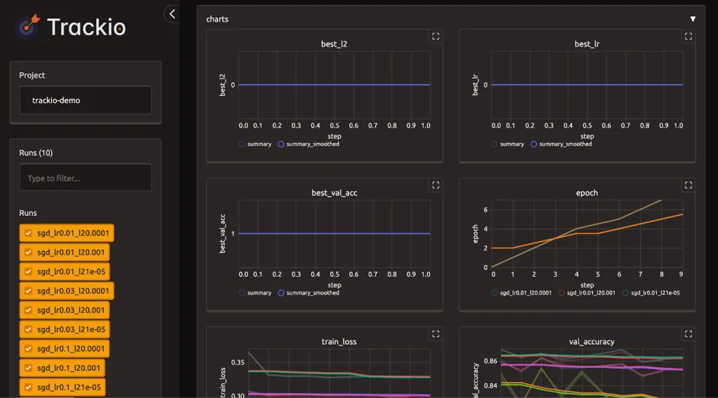
Trackio Dashboard Overview
In conclusion, we experience how Trackio streamlines experiment tracking without the complexity of heavy infrastructure or API setups. We not only log and compare runs but also capture structured results, import external data, and launch an interactive dashboard directly inside Colab. With this workflow, we see how Trackio empowers us to stay organized, monitor progress effectively, and make better decisions during experimentation. This tutorial gives us a strong foundation to integrate Trackio into our own machine learning projects seamlessly.
Check out the . Feel free to check out our . Also, feel free to follow us on and don’t forget to join our and Subscribe to .
The post appeared first on .